ggplot(chic, aes(x = date, y = temp, color = o3)) +
  geom_point() +
  geom_hline(yintercept = c(0, 73)) +
  labs(x = "Year", y = "Temperature (°F)")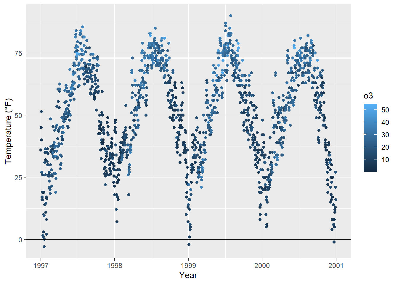
You might want to highlight a given range or threshold, which can be done plotting a line at defined coordinates using geom_hline() (for “horizontal lines”) or geom_vline() (for “vertical lines”):
ggplot(chic, aes(x = date, y = temp, color = o3)) +
geom_point() +
geom_hline(yintercept = c(0, 73)) +
labs(x = "Year", y = "Temperature (°F)")
g <- ggplot(chic, aes(x = temp, y = dewpoint)) +
  geom_point(color = "dodgerblue", alpha = .5) +
  labs(x = "Temperature (°F)", y = "Dewpoint")

g +
  geom_vline(aes(xintercept = median(temp)), linewidth = 1.5,
             color = "firebrick", linetype = "dashed") +
  geom_hline(aes(yintercept = median(dewpoint)), linewidth = 1.5,
             color = "firebrick", linetype = "dashed")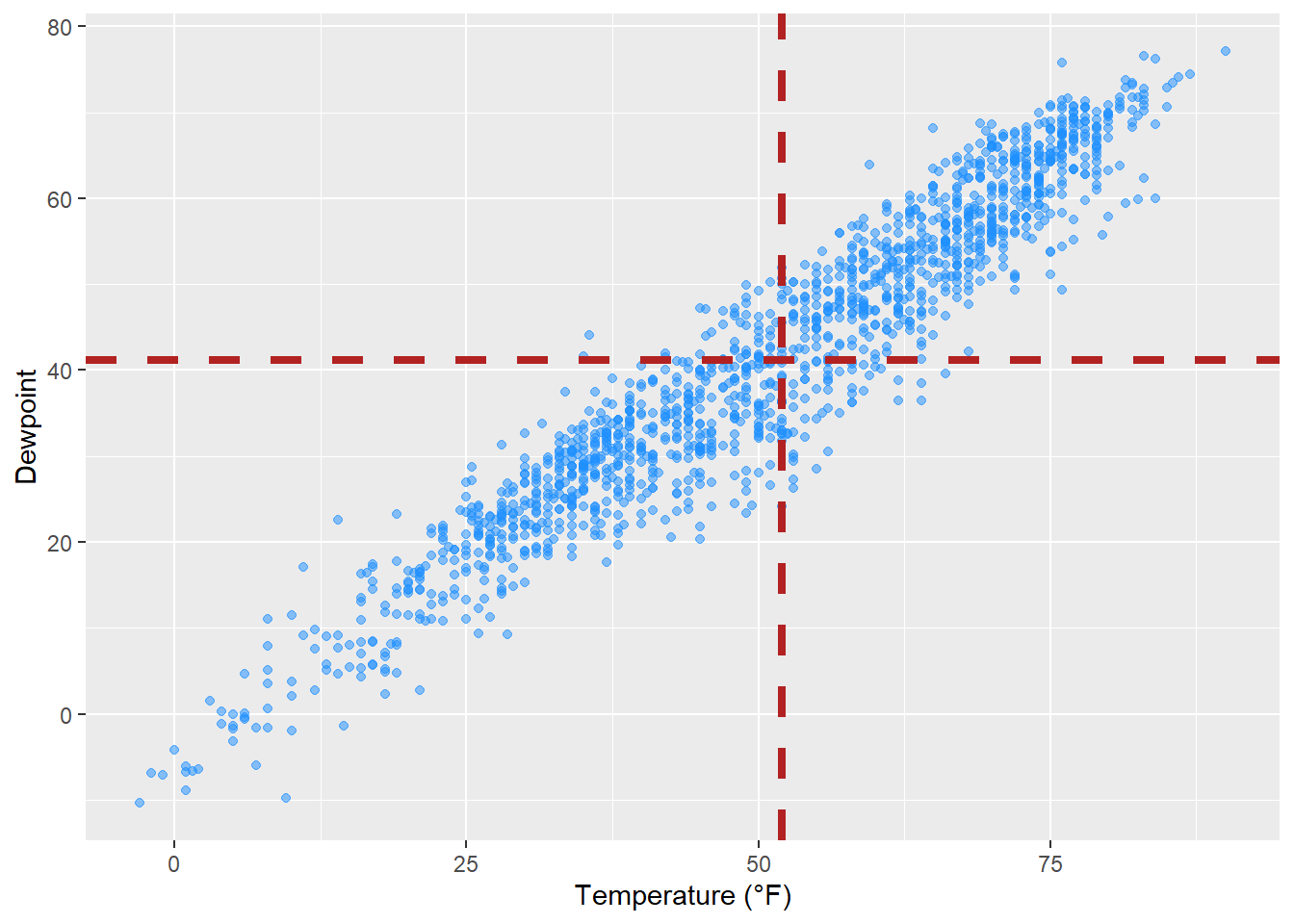
If you want to add a line with a slope not being 0 or 1, respectively, you need to use geom_abline(). This is for example the case if you want to add a regression line using the arguments intercept and slope:
reg <- lm(dewpoint ~ temp, data = chic)

g +
  geom_abline(intercept = coefficients(reg)[1],
              slope = coefficients(reg)[2],
              color = "darkorange2",
              linewidth = 1.5) +
  labs(title = paste0("y = ", round(coefficients(reg)[2], 2),
                      " * x + ", round(coefficients(reg)[1], 2)))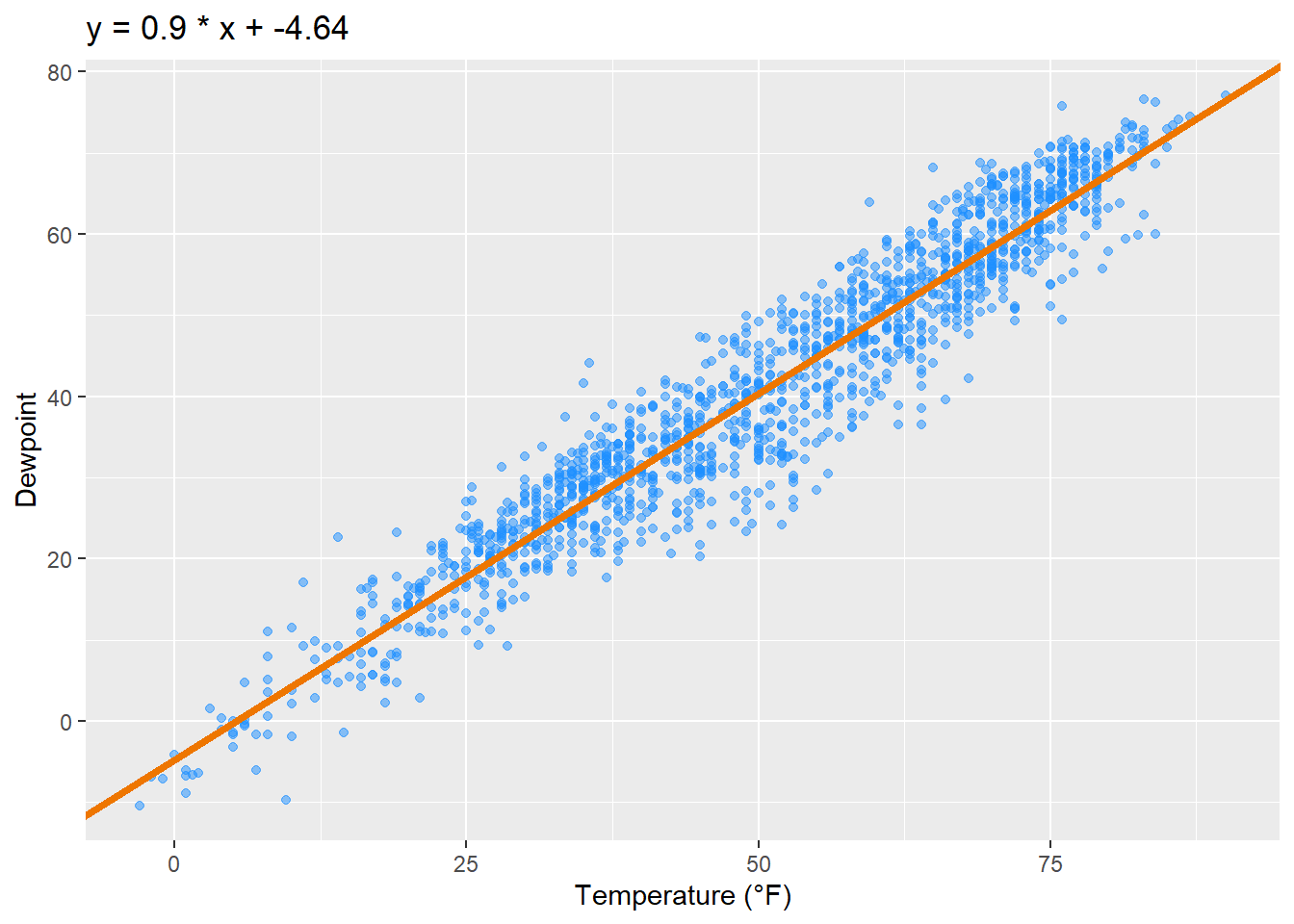
Later, we will learn how to add a linear fit with one command using stat_smooth(method = "lm"). However, there might be other reasons to add a line with a given slope and this is how one does it 🤷
The previous approaches always covered the whole range of the plot panel, but sometimes one wants to highlight only a given area or use lines for annotations. In this case, geom_linerange() is here to help:
g +
  ## vertical line
  geom_linerange(aes(x = 50, ymin = 20, ymax = 55),
                 color = "steelblue", linewidth = 2) +
  ## horizontal line
  geom_linerange(aes(xmin = -Inf, xmax = 25, y = 0),
                 color = "red", linewidth = 1)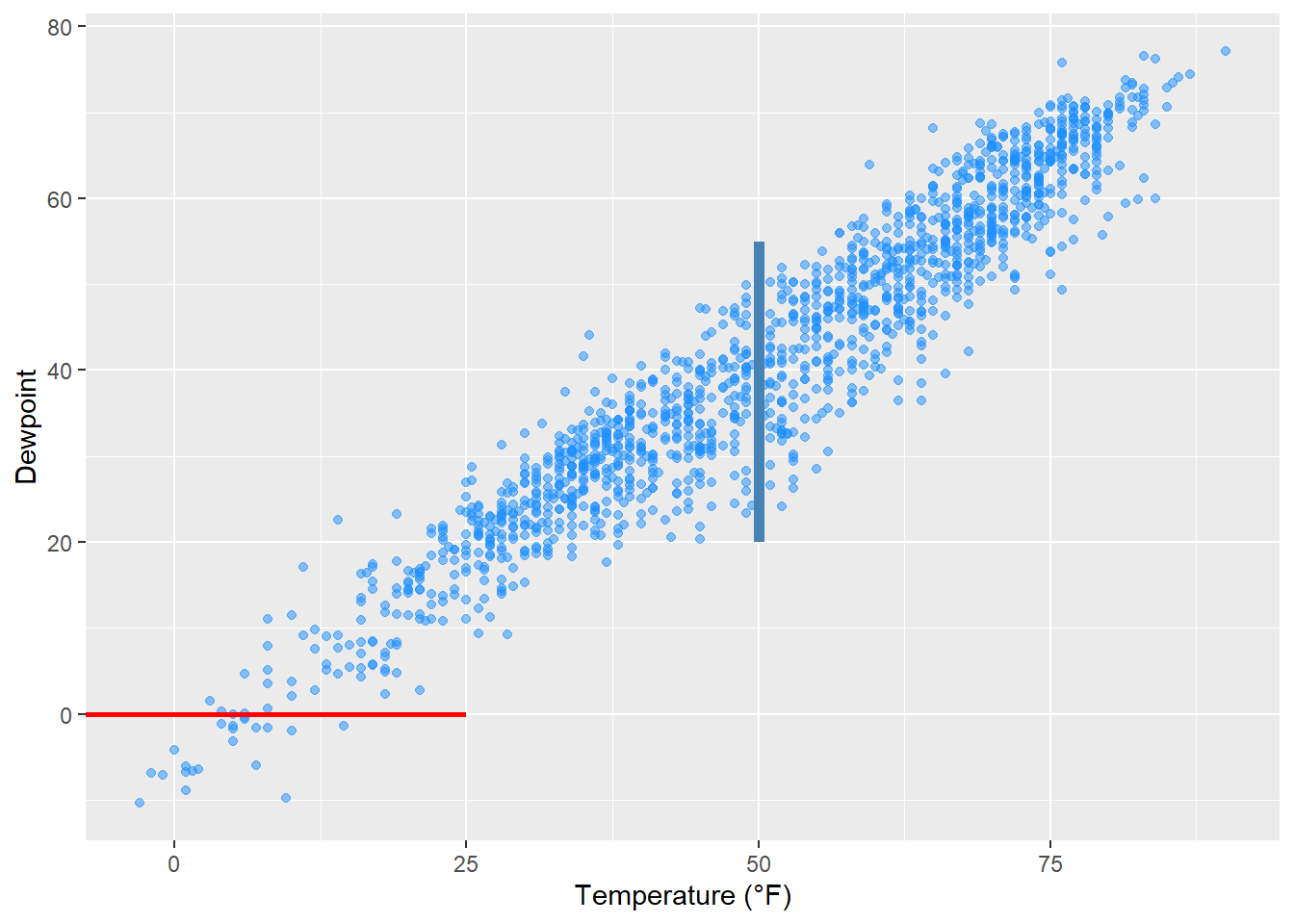
Or you can use annotate(geom = "segment") to draw lines with a slope differing from 0 and 1:
g +
  annotate(geom = "segment",
           x = 50, xend = 75,
                   y = 20, yend = 45,
               color = "purple", linewidth = 2)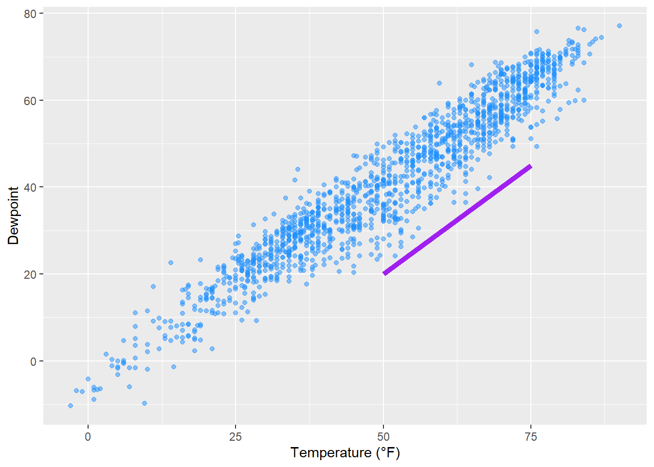
annotate(geom = "curve") adds curves. Well, and straight lines if you like:
g +
  annotate(geom = "curve",x = 0, y = 60, xend = 75, yend = 0,
             color = "tan", linewidth = 2) +
  annotate(geom = "curve",
           x = 0, y = 60, xend = 75, yend = 0,
             curvature = -0.7, angle = 45,
             color = "darkgoldenrod1", linewidth = 1) +
  annotate(geom = "curve", x = 0, y = 60, xend = 75, yend = 0,
             curvature = 0, linewidth = 1.5)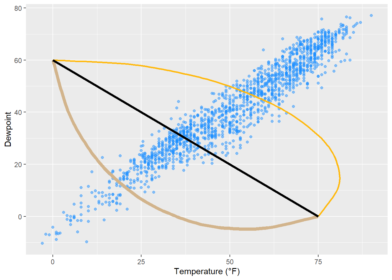
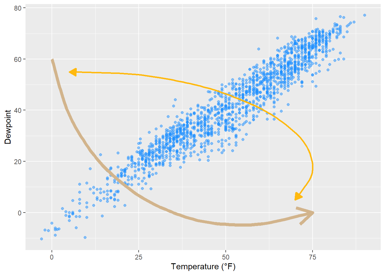
The same geom can be used to draw arrows:
g +
  annotate(geom = "curve", x = 0, y = 60, xend = 75, yend = 0,
             color = "tan", linewidth = 2,
             arrow = arrow(length = unit(0.07, "npc"))) +
  annotate(geom = "curve", x = 5, y = 55, xend = 70, yend = 5,
             curvature = -0.7, angle = 45,
             color = "darkgoldenrod1", linewidth = 1,
             arrow = arrow(length = unit(0.03, "npc"),
                           type = "closed",
                           ends = "both"))