17  Working with Smoothings

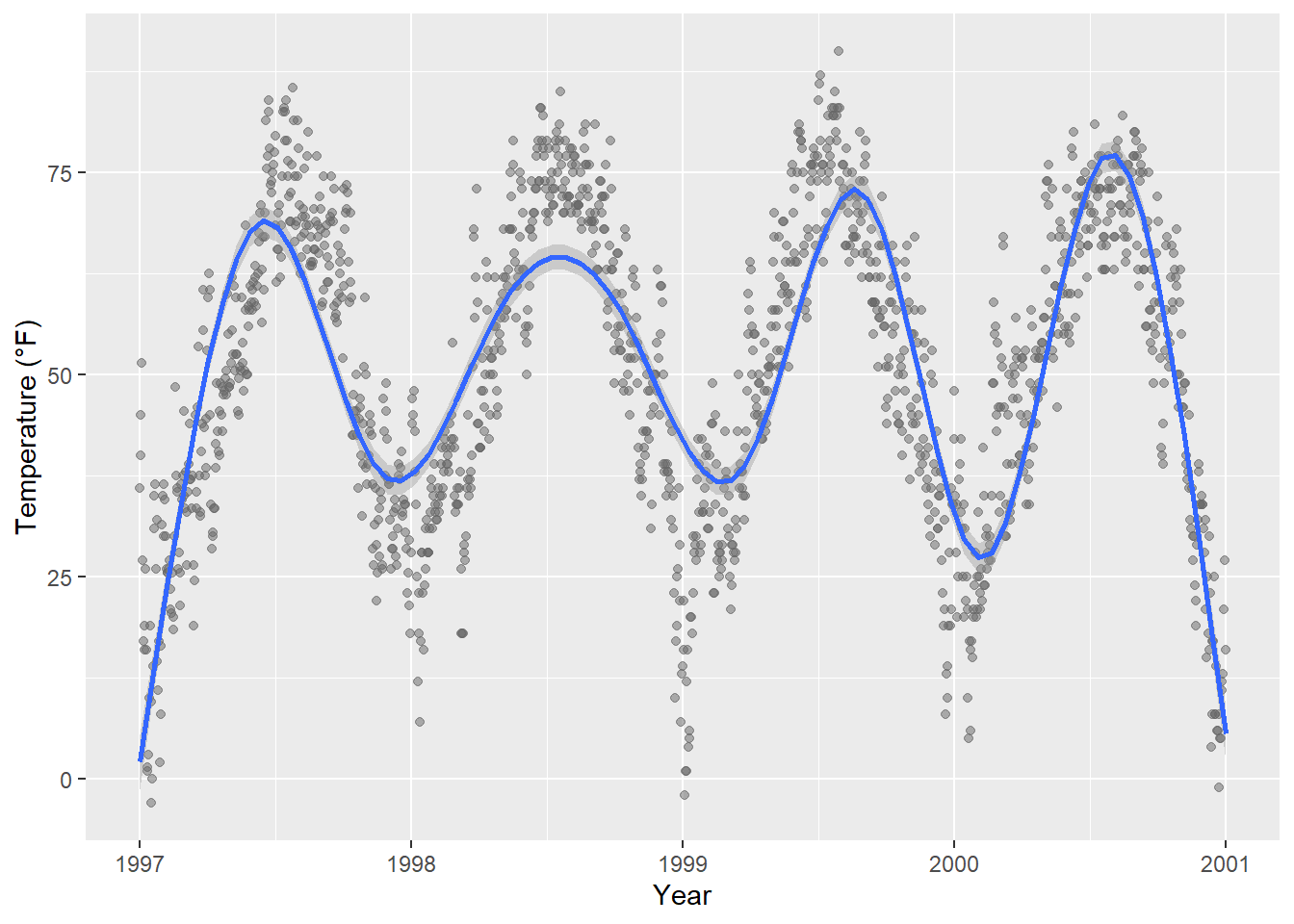
It is amazingly easy to add smoothing to your data using {ggplot2}.

17.1 Default: Adding a LOESS or GAM Smoothing

You can simply use stat_smooth()—not even a formula is required. This adds a LOESS (locally weighted scatter plot smoothing, method = "loess") if you have fewer than 1000 points or a GAM (generalized additive model, method = "gam") otherwise. Since we have more than 1000 points, the smoothing is based on a GAM:

ggplot(chic, aes(x = date, y = temp)) +
  geom_point(color = "gray40", alpha = .5) +
  stat_smooth() +
  labs(x = "Year", y = "Temperature (°F)") 

`geom_smooth()` using method = 'gam' and formula = 'y ~ s(x, bs = "cs")'

Note

In most cases one wants the points to be on top of the ribbon so make sure you always call the smoothing before you add the points.

17.2 Adding a Linear Fit

Though the default is a LOESS or GAM smoothing, it is also easy to add a standard linear fit:

ggplot(chic, aes(x = temp, y = dewpoint)) +
   geom_point(color = "gray40", alpha = .5) +
   stat_smooth(method = "lm", se = FALSE,
               color = "firebrick", linewidth = 1.3) +
   labs(x = "Temperature (°F)", y = "Dewpoint")

`geom_smooth()` using formula = 'y ~ x'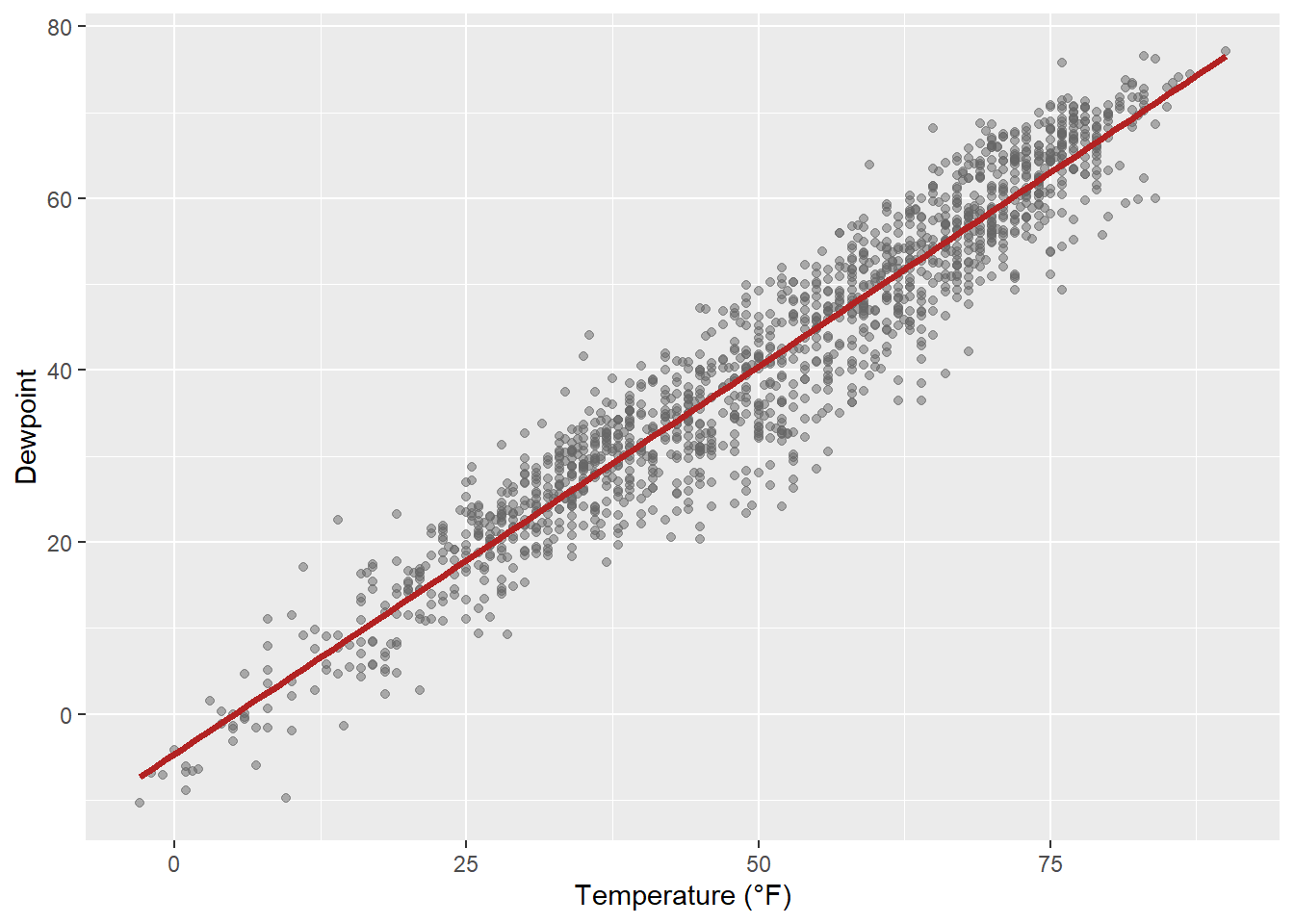

17.3 Specifying the Formula for Smoothing

{ggplot2} allows you to specify the model you want it to use. Maybe you want to use a polynomial regression?

ggplot(chic, aes(x = o3, y = temp)) +
  geom_point(color = "gray40", alpha = .3) +
  geom_smooth(
    method = "lm",
    formula = y ~ x + I(x^2) + I(x^3) + I(x^4) + I(x^5),
    color = "black",
    fill = "firebrick"
  ) +
  labs(x = "Ozone Level", y = "Temperature (°F)")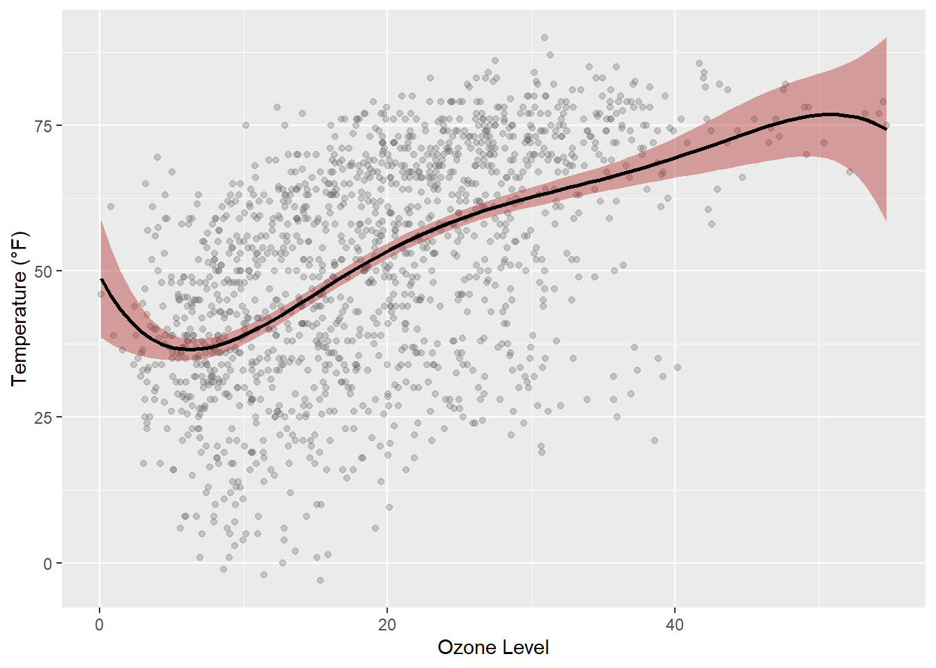

Difference between geom and stat

Huh, geom_smooth()? There is an important difference between geom and stat but here it really doesn’t matter which one you use. Expand to compare both.

ggplot(chic, aes(x = o3, y = temp)) +
  geom_point(color = "gray40", alpha = .3) +
  geom_smooth(stat = "smooth") + ## the default
  labs(x = "Ozone Level", y = "Temperature (°F)")

`geom_smooth()` using method = 'gam' and formula = 'y ~ s(x, bs = "cs")'

ggplot(chic, aes(x = o3, y = temp)) +
  geom_point(color = "gray40", alpha = .3) +
  stat_smooth(geom = "smooth") + ## the default
  labs(x = "Ozone Level", y = "Temperature (°F)")

`geom_smooth()` using method = 'gam' and formula = 'y ~ s(x, bs = "cs")'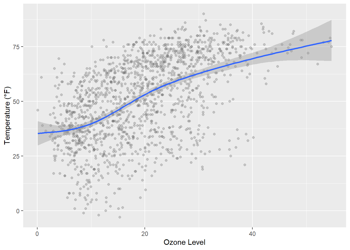

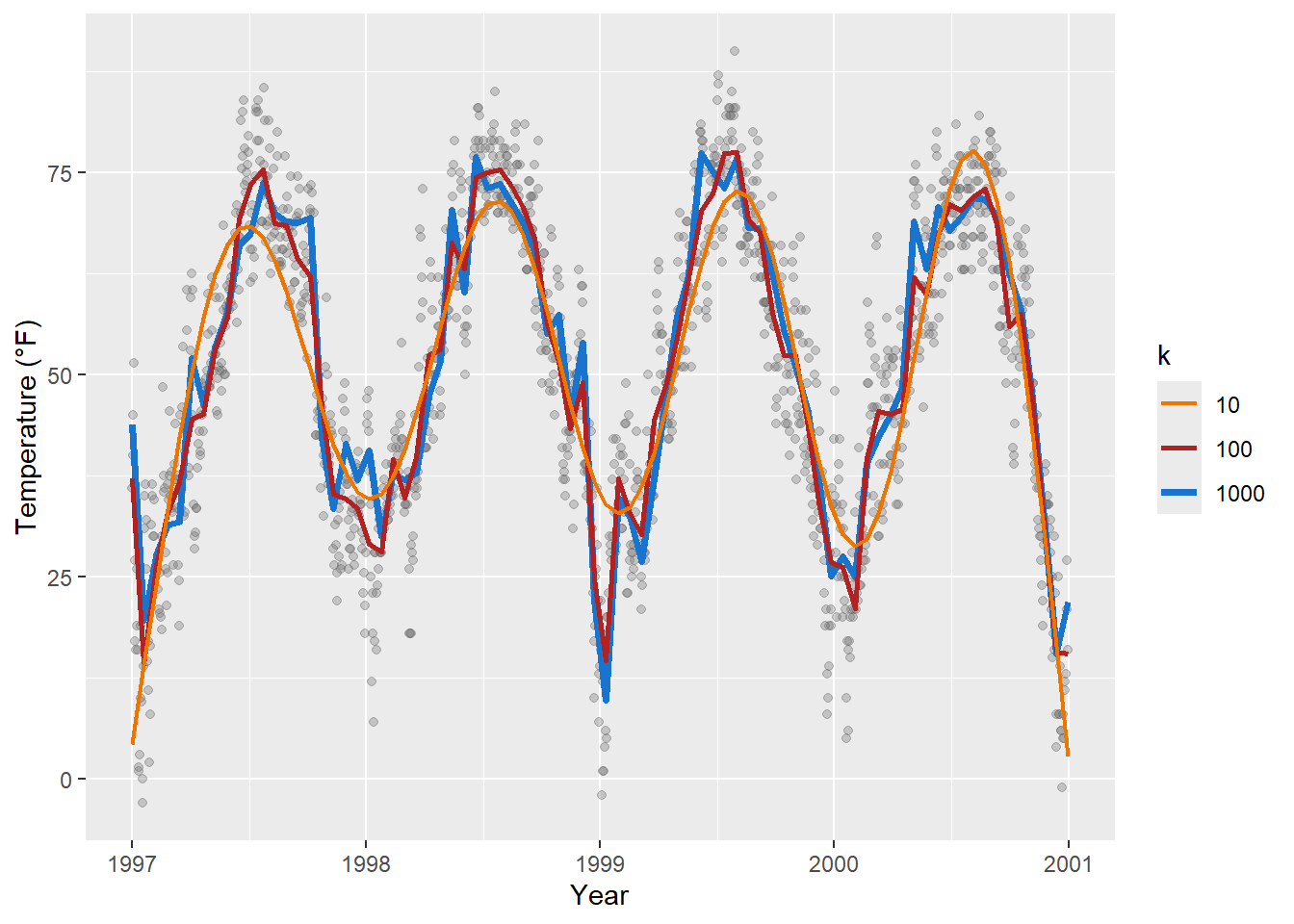
Or lets say you want to increase the GAM dimension (add some additional wiggles to the smooth):

cols <- c("darkorange2", "firebrick", "dodgerblue3")

ggplot(chic, aes(x = date, y = temp)) +
  geom_point(color = "gray40", alpha = .3) +
  stat_smooth(aes(col = "1000"),
              method = "gam",
              formula = y ~ s(x, k = 1000),
              se = FALSE, linewidth = 1.3) +
  stat_smooth(aes(col = "100"),
              method = "gam",
              formula = y ~ s(x, k = 100),
              se = FALSE, linewidth = 1) +
  stat_smooth(aes(col = "10"),
              method = "gam",
              formula = y ~ s(x, k = 10),
              se = FALSE, linewidth = .8) +
  scale_color_manual(name = "k", values = cols) +
  labs(x = "Year", y = "Temperature (°F)")