ggplot(chic, aes(x = date, y = temp)) +
  geom_point(color = "firebrick") +
  labs(x = "Year", y = "Temperature (°F)")
To add clear and descriptive labels to the axes, we can utilize the labs() function. This function allows us to provide a character string for each label we wish to modify, such as x and y:
ggplot(chic, aes(x = date, y = temp)) +
geom_point(color = "firebrick") +
labs(x = "Year", y = "Temperature (°F)")
xlab() and ylab()
You also can add axis titles by using xlab() and ylab(). Click to see example.
ggplot(chic, aes(x = date, y = temp)) +
  geom_point(color = "firebrick") +
  xlab("Year") +
  ylab("Temperature (°F)")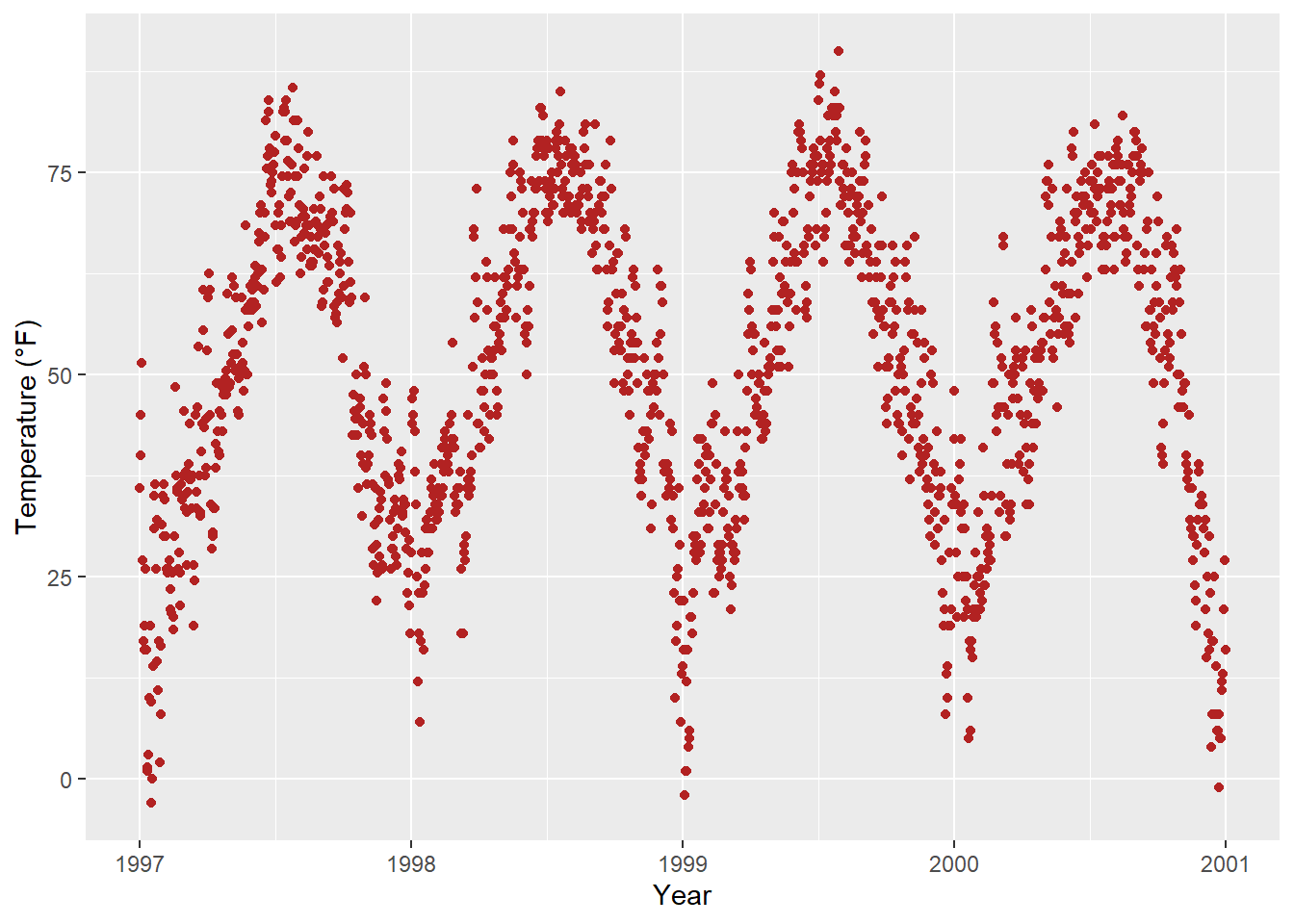
Typically, you can specify symbols by directly adding the symbol itself (e.g., “°”). However, the code below also enables the addition of not only symbols but also features like superscripts:
ggplot(chic, aes(x = date, y = temp)) +
  geom_point(color = "firebrick") +
  labs(x = "Year", y = expression(paste("Temperature (", degree ~ F, ")"^"(Hey, why should we use metric units?!)")))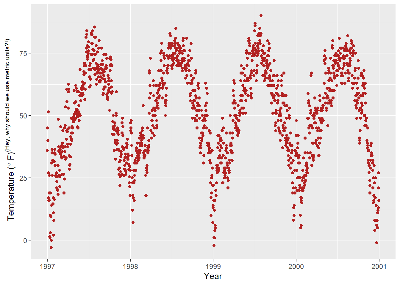
theme() is a crucial command for adjusting specific theme elements such as texts, titles, boxes, symbols, backgrounds, and more. We’ll be utilizing this command extensively! Initially, we’ll focus on modifying text elements. We can customize the properties of all text elements or specific ones, such as axis titles, by overriding the default element_text() within the theme() call:
ggplot(chic, aes(x = date, y = temp)) +
  geom_point(color = "firebrick") +
  labs(x = "Year", y = "Temperature (°F)") +
  theme(axis.title.x = element_text(vjust = 0, size = 15),
        axis.title.y = element_text(vjust = 2, size = 15))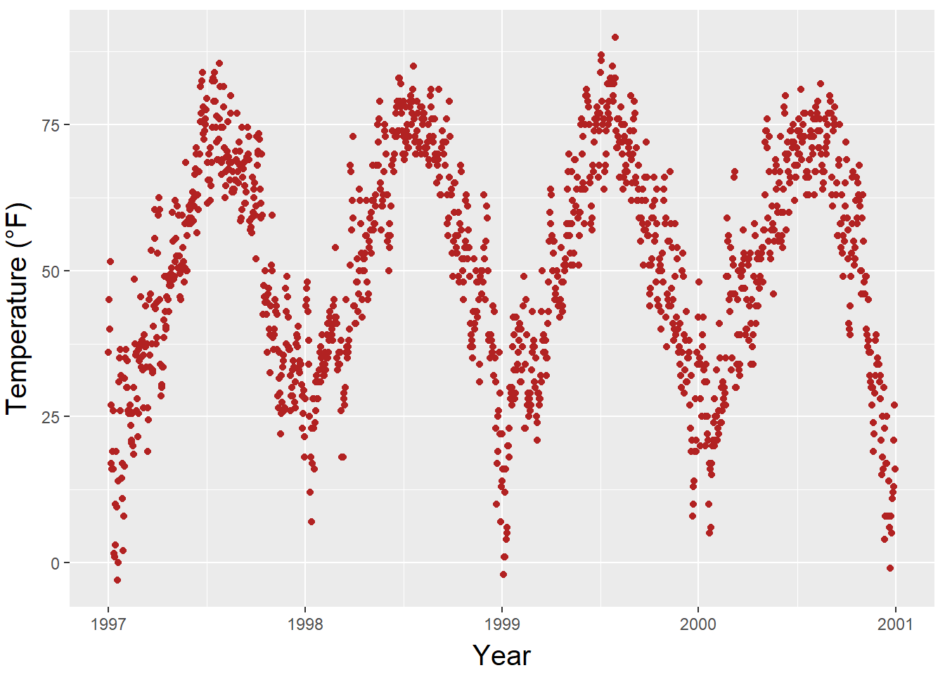
The vjust parameter controls vertical alignment and typically ranges between 0 and 1, but you can also specify values outside that range. It’s worth noting that even when adjusting the position of the axis title along the y-axis horizontally, we still need to specify vjust (which is correct from the perspective of the label’s alignment). Additionally, you can modify the distance by specifying the margin for both text elements:
ggplot(chic, aes(x = date, y = temp)) +
  geom_point(color = "firebrick") +
  labs(x = "Year", y = "Temperature (°F)") +
  theme(axis.title.x = element_text(margin = margin(t = 10), size = 15),
        axis.title.y = element_text(margin = margin(r = 10), size = 15))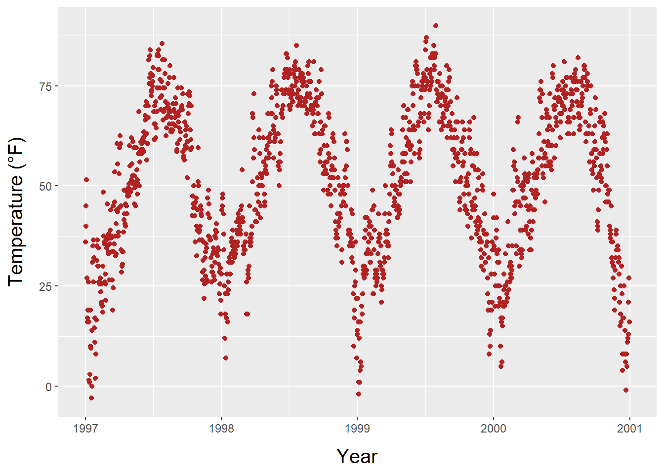
The labels t and r within the margin() object correspond to top and right, respectively. Alternatively, you can specify all four margins using margin(t, r, b, l). It’s important to note that we need to adjust the right margin to modify the space on the y-axis, not the bottom margin.
A helpful mnemonic for remembering the order of the margin sides is “t-r-ou-b-l-e”.
Once more, we utilize the theme() function to modify the axis.title element and/or its subordinated elements, axis.title.x and axis.title.y. Within the element_text() function, we can override defaults for properties such as size, color, and face:
ggplot(chic, aes(x = date, y = temp)) +
  geom_point(color = "firebrick") +
  labs(x = "Year", y = "Temperature (°F)") +
  theme(axis.title = element_text(size = 15, color = "firebrick",
                                  face = "italic"))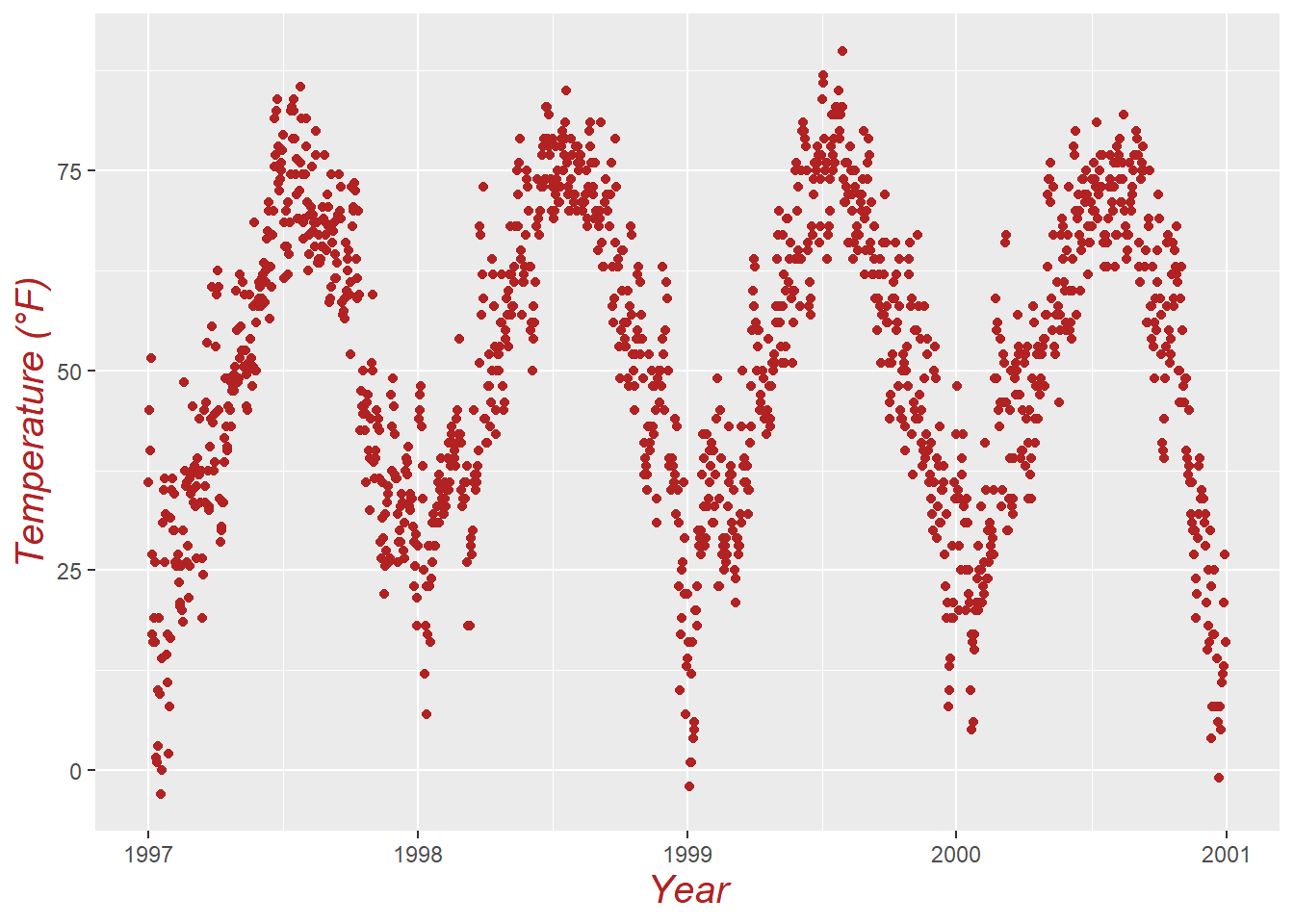
The face argument can be used to make the font bold or italic or even bold.italic.
ggplot(chic, aes(x = date, y = temp)) +
  geom_point(color = "firebrick") +
  labs(x = "Year", y = "Temperature (°F)") +
  theme(axis.title.x = element_text(color = "sienna", size = 15),
        axis.title.y = element_text(color = "orangered", size = 15))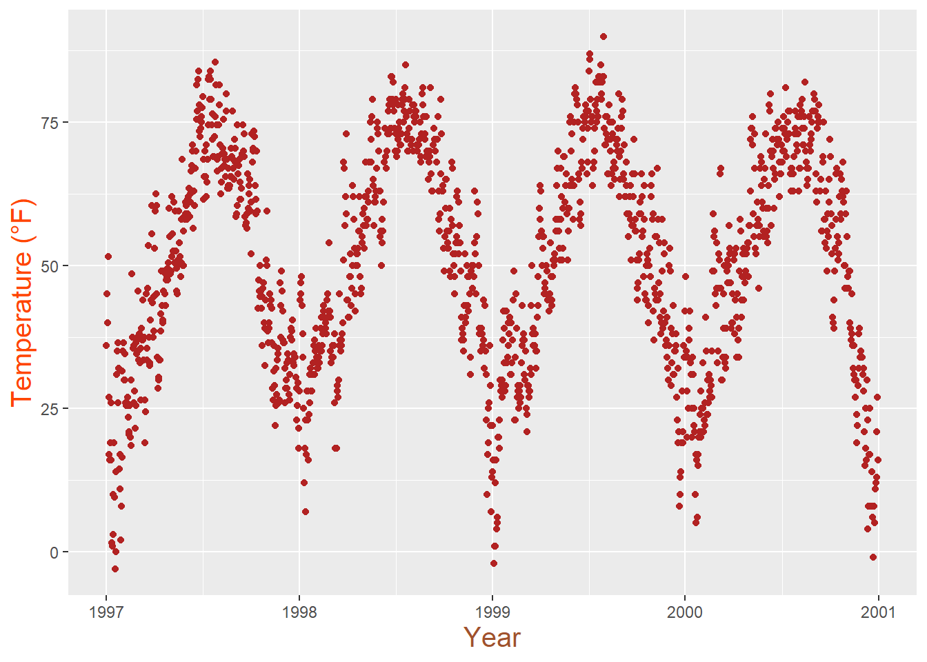
You could also employ a combination of axis.title and axis.title.y, as axis.title.x inherits values from axis.title. Expand to See the example below:
ggplot(chic, aes(x = date, y = temp)) +
  geom_point(color = "firebrick") +
  labs(x = "Year", y = "Temperature (°F)") +
  theme(axis.title = element_text(color = "sienna", size = 15),
        axis.title.y = element_text(color = "orangered", size = 15))
You can adjust some properties for both axis titles simultaneously, while modifying others exclusively for one axis or individual properties for each axis title:
ggplot(chic, aes(x = date, y = temp)) +
  geom_point(color = "firebrick") +
  labs(x = "Year", y = "Temperature (°F)") +
  theme(axis.title = element_text(color = "sienna", size = 15, face = "bold"),
        axis.title.y = element_text(face = "bold.italic"))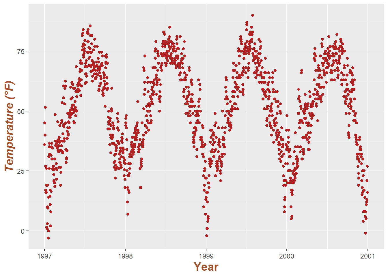
Likewise, you can alter the appearance of the axis text (i.e., the numbers) by utilizing axis.text and/or its subordinated elements, axis.text.x and axis.text.y:
ggplot(chic, aes(x = date, y = temp)) +
  geom_point(color = "firebrick") +
  labs(x = "Year", y = "Temperature (°F)") +
  theme(axis.text = element_text(color = "dodgerblue", size = 12),
        axis.text.x = element_text(face = "italic"))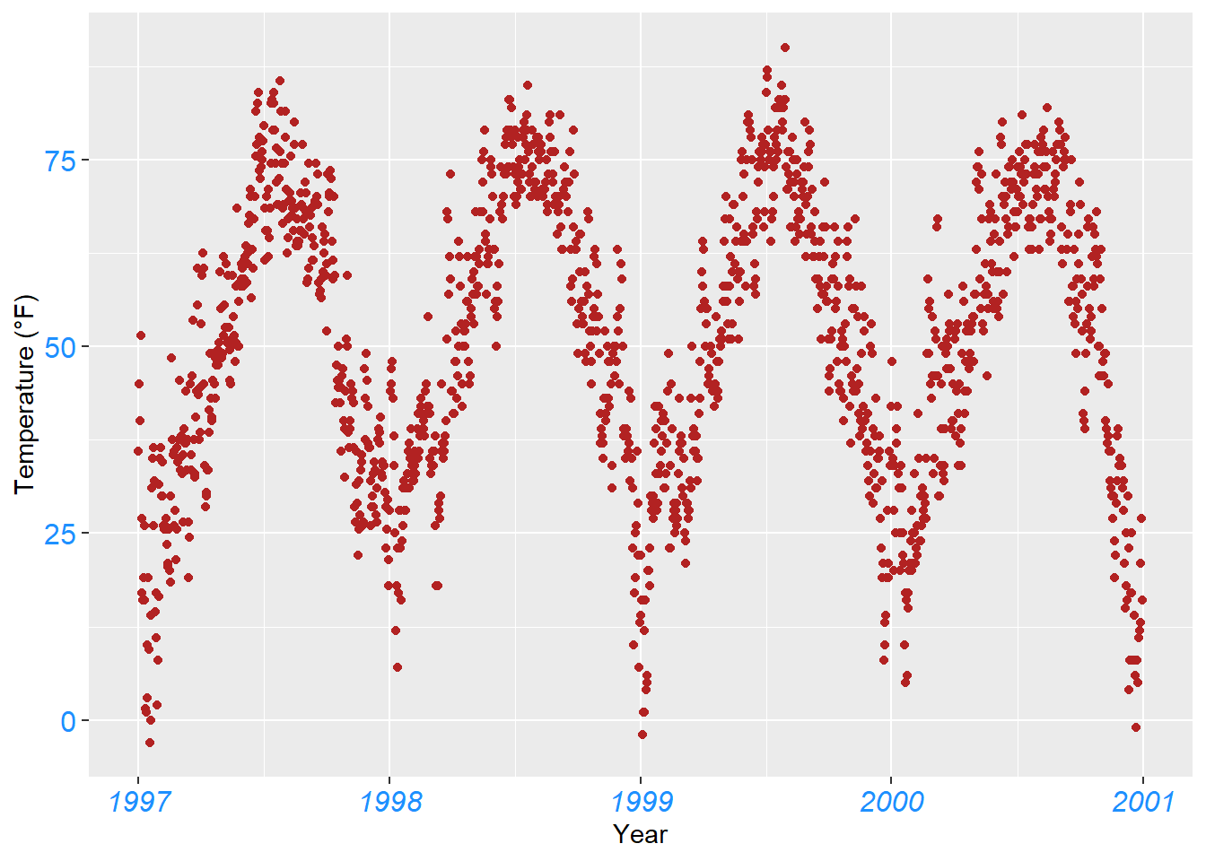
You can rotate any text elements by specifying an angle. Subsequently, you can adjust the position of the text horizontally (0 = left, 1 = right) and vertically (0 = top, 1 = bottom) using hjust and vjust:
ggplot(chic, aes(x = date, y = temp)) +
  geom_point(color = "firebrick") +
  labs(x = "Year", y = "Temperature (°F)") +
  theme(axis.text.x = element_text(angle = 50, vjust = 1, hjust = 1, size = 12))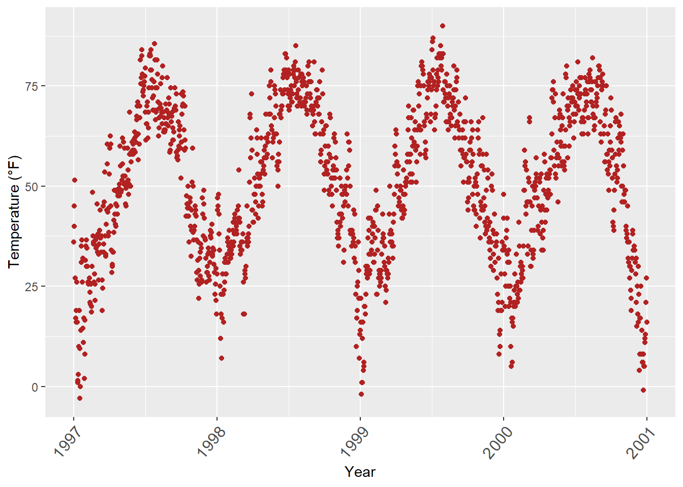
There might be rare occasions where you need to remove axis text and ticks. Here’s how you can achieve it:
ggplot(chic, aes(x = date, y = temp)) +
  geom_point(color = "firebrick") +
  labs(x = "Year", y = "Temperature (°F)") +
  theme(axis.ticks.y = element_blank(),
        axis.text.y = element_blank())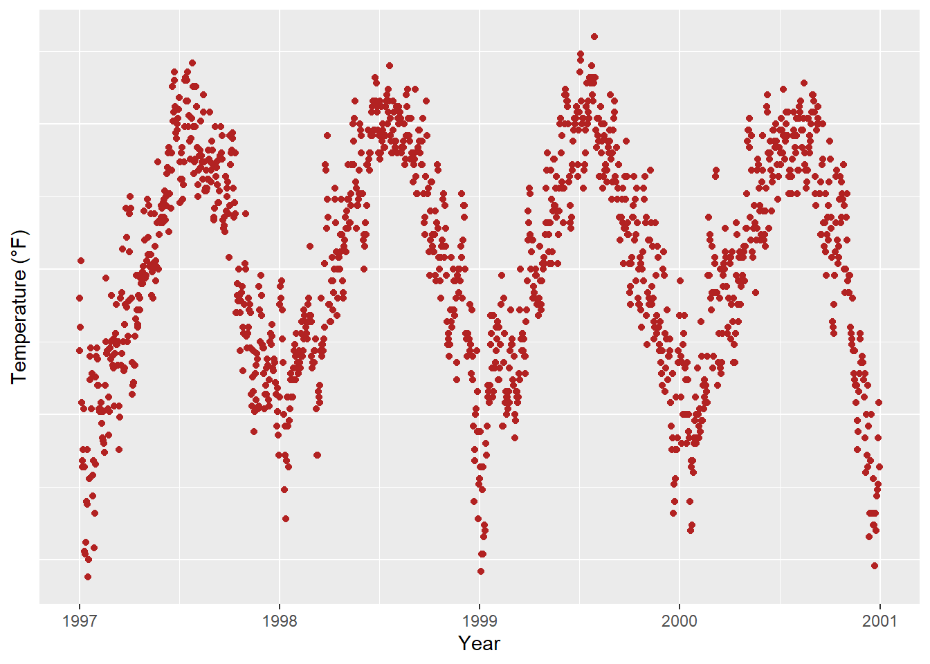
I’ve introduced three theme elements—text, lines, and rectangles—but there’s actually one more: element_blank(), which removes the element entirely. However, it’s not considered an official element like the others.
If you wish to remove a theme element entirely, you can always use element_blank().
We can use theme_blank(), but it’s much simpler to just omit the label in the labs() (or xlab()) call:
ggplot(chic, aes(x = date, y = temp)) +
  geom_point(color = "firebrick") +
  labs(x = NULL, y = "")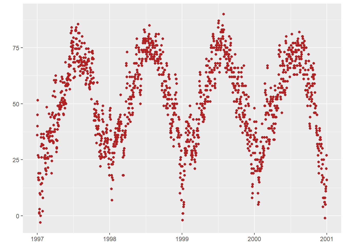
Note that NULL removes the element (similarly to element_blank()), while empty quotes "" will keep the spacing for the axis title but print nothing.
Occasionally, you may want to focus on a specific range of your data without altering the dataset itself. You can accomplish this with ease:
ggplot(chic, aes(x = date, y = temp)) +
  geom_point(color = "firebrick") +
  labs(x = "Year", y = "Temperature (°F)") +
  ylim(c(0, 50))
Warning: Removed 777 rows containing missing values or values outside the scale range
(`geom_point()`).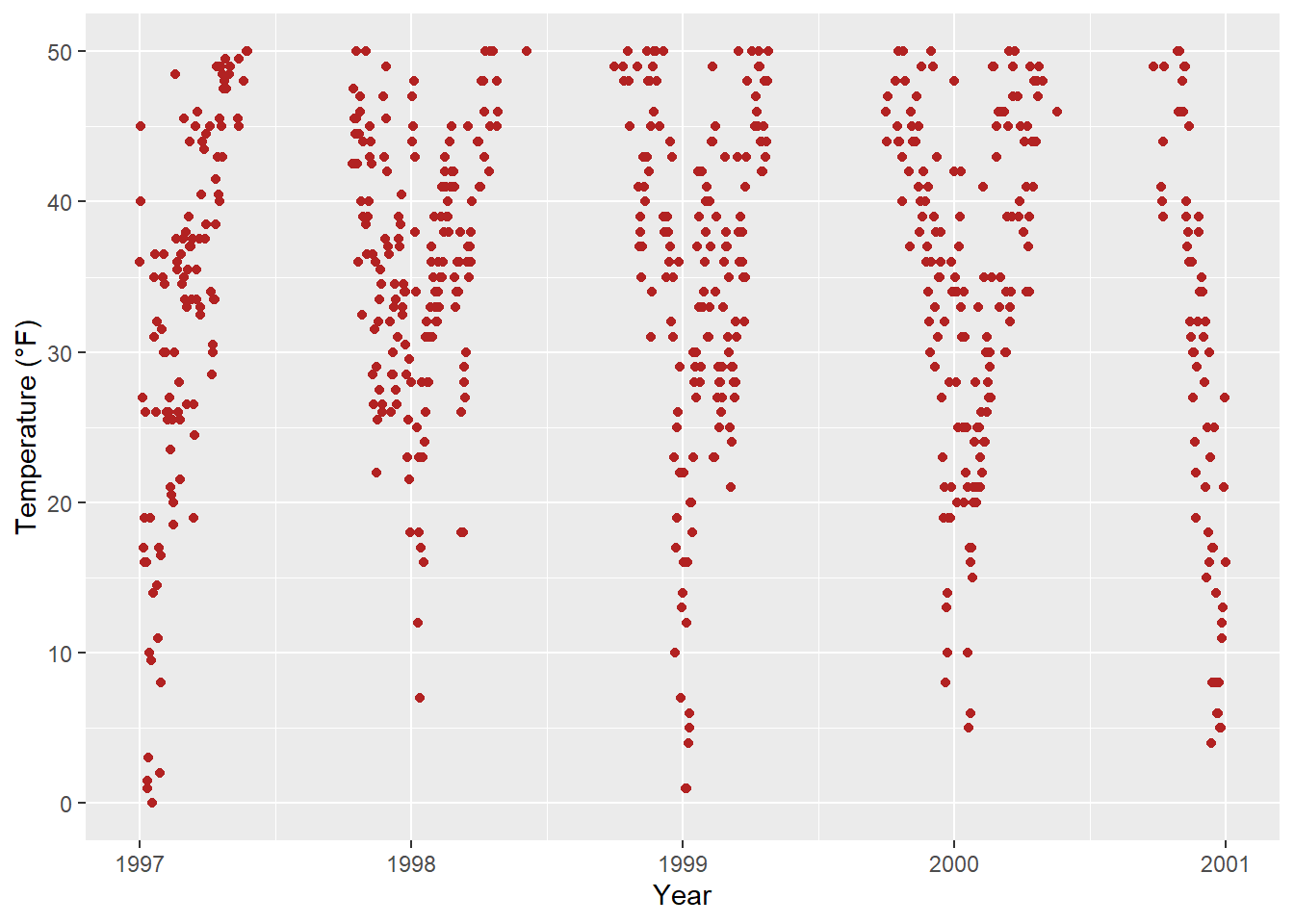
Alternatively, you can utilize scale_y_continuous(limits = c(0, 50)) or coord_cartesian(ylim = c(0, 50)). The former removes all data points outside the specified range, while the latter adjusts the visible area, similar to ylim(c(0, 50)). At first glance, it may seem that both approaches yield the same result. However, there is an important distinction—compare the following two plots:
Warning: Removed 777 rows containing missing values or values outside the scale range
(`geom_point()`).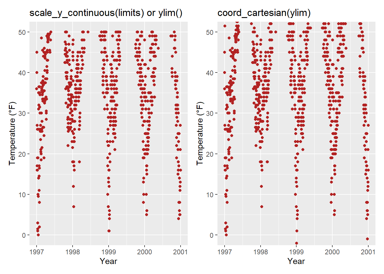
You may have noticed that on the left, there is some empty buffer around your y limits, while on the right, points are plotted right up to the border and even beyond. This effectively illustrates the concept of subsetting (left) versus zooming (right). To demonstrate why this distinction is significant, let’s examine a different chart type: a box plot.
Warning: Removed 777 rows containing non-finite outside the scale range
(`stat_boxplot()`).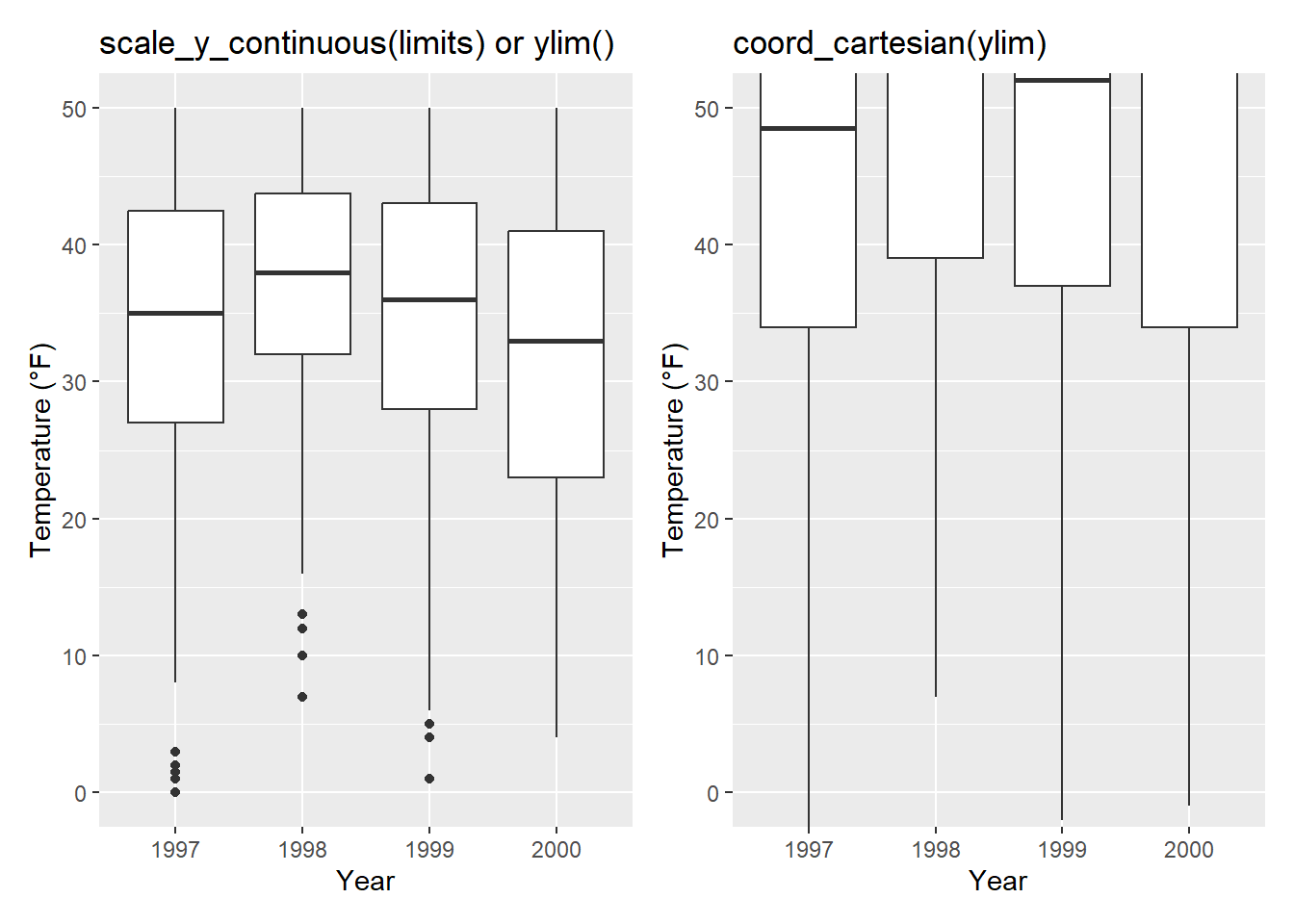
Indeed, because scale_x|y_continuous() subsets the data first, we obtain completely different (and potentially incorrect, especially if this was not our intention) estimates for the box plots! This realization highlights the importance of ensuring data integrity throughout the plotting process. It’s crucial to avoid inadvertently manipulating the data while plotting, as it could lead to inaccurate summary statistics reported in your report, paper, or thesis.
Related to that, you can instruct R to plot the graph starting at the origin:
chic_high <- dplyr::filter(chic, temp > 25, o3 > 20)

ggplot(chic_high, aes(x = temp, y = o3)) +
  geom_point(color = "darkcyan") +
  labs(x = "Temperature higher than 25°F",
       y = "Ozone higher than 20 ppb") +
  expand_limits(x = 0, y = 0)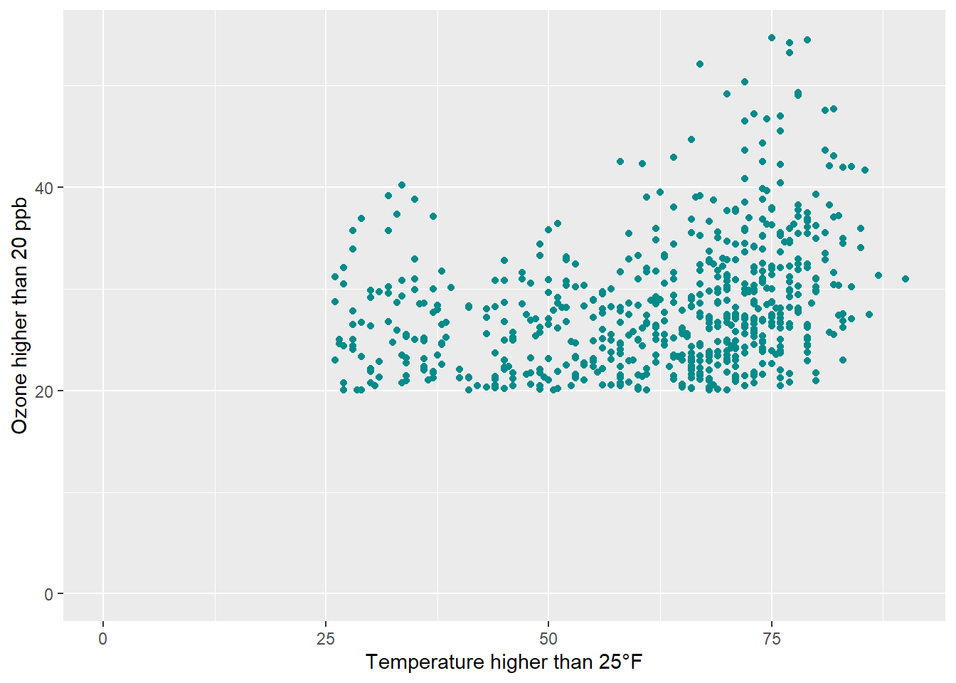
coord_cartesian(xlim = c(0, NA), ylim = c(0, NA))
Using coord_cartesian(xlim = c(0, NA), ylim = c(0, NA)) will produce the same result. CLICK to See the example below:
chic_high <- dplyr::filter(chic, temp > 25, o3 > 20)

ggplot(chic_high, aes(x = temp, y = o3)) +
  geom_point(color = "darkcyan") +
  labs(x = "Temperature higher than 25°F",
       y = "Ozone higher than 20 ppb") +
  coord_cartesian(xlim = c(0, NA), ylim = c(0, NA))
But we can also ensure that it truly starts at the origin!
ggplot(chic_high, aes(x = temp, y = o3)) +
  geom_point(color = "darkcyan") +
  labs(x = "Temperature higher than 25°F",
       y = "Ozone higher than 20 ppb") +
  expand_limits(x = 0, y = 0) +
  coord_cartesian(expand = FALSE, clip = "off")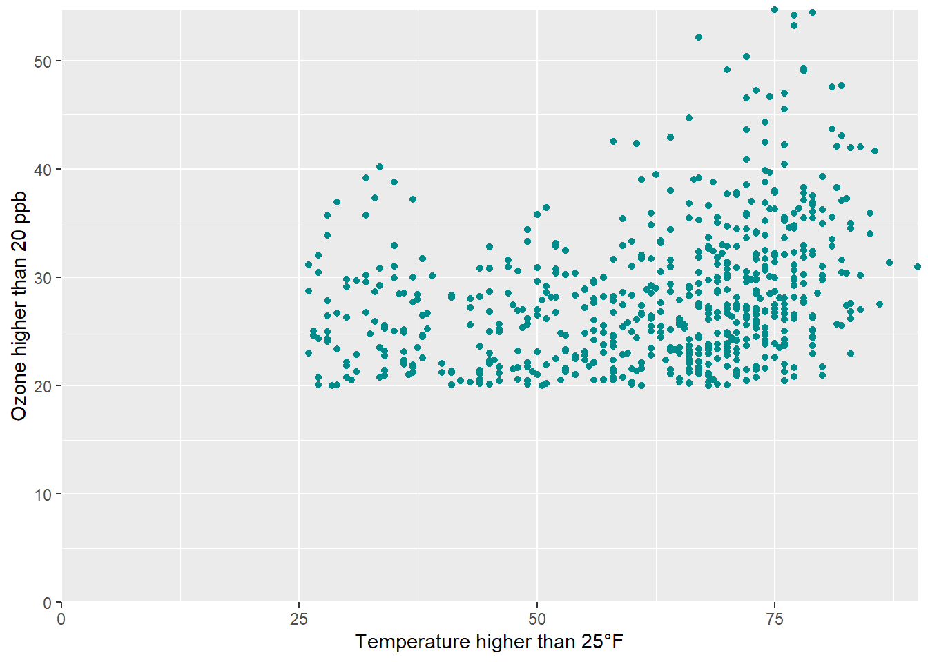
The clip = "off" argument in any coordinate system, always starting with coord_*, enables drawing outside of the panel area.
Here, I invoke it to ensure that the tick marks at c(0, 0) remain intact and are not truncated. For further insights, refer to the Twitter thread by Claus Wilke.
For demonstration purposes, let’s plot temperature against temperature with some random noise. The coord_equal() function provides a coordinate system with a specified ratio, representing the number of units on the y-axis equivalent to one unit on the x-axis. By default, ratio = 1 ensures that one unit on the x-axis is the same length as one unit on the y-axis:
ggplot(chic, aes(x = temp, y = temp + rnorm(nrow(chic), sd = 20))) +
  geom_point(color = "sienna") +
  labs(x = "Temperature (°F)", y = "Temperature (°F) + random noise") +
  xlim(c(0, 100)) + ylim(c(0, 150)) +
  coord_fixed()
Warning: Removed 48 rows containing missing values or values outside the scale range
(`geom_point()`).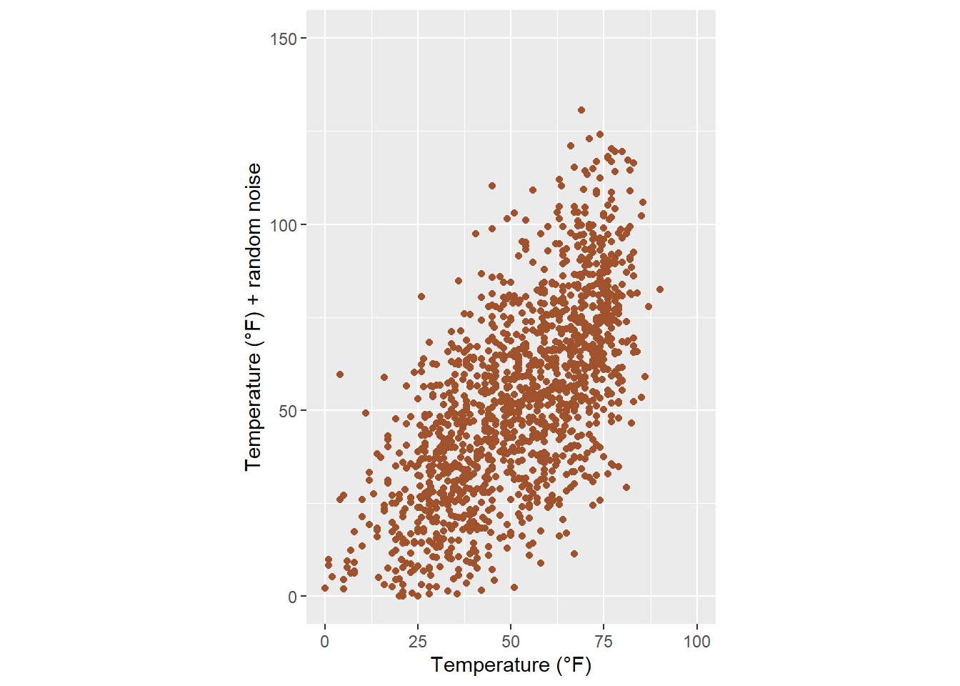
Ratios higher than one result in units on the y-axis being longer than units on the x-axis, while ratios lower than one have the opposite effect:
ggplot(chic, aes(x = temp, y = temp + rnorm(nrow(chic), sd = 20))) +
  geom_point(color = "sienna") +
  labs(x = "Temperature (°F)", y = "Temperature (°F) + random noise") +
  xlim(c(0, 100)) + ylim(c(0, 150)) +
  coord_fixed(ratio = 1/5)
Warning: Removed 47 rows containing missing values or values outside the scale range
(`geom_point()`).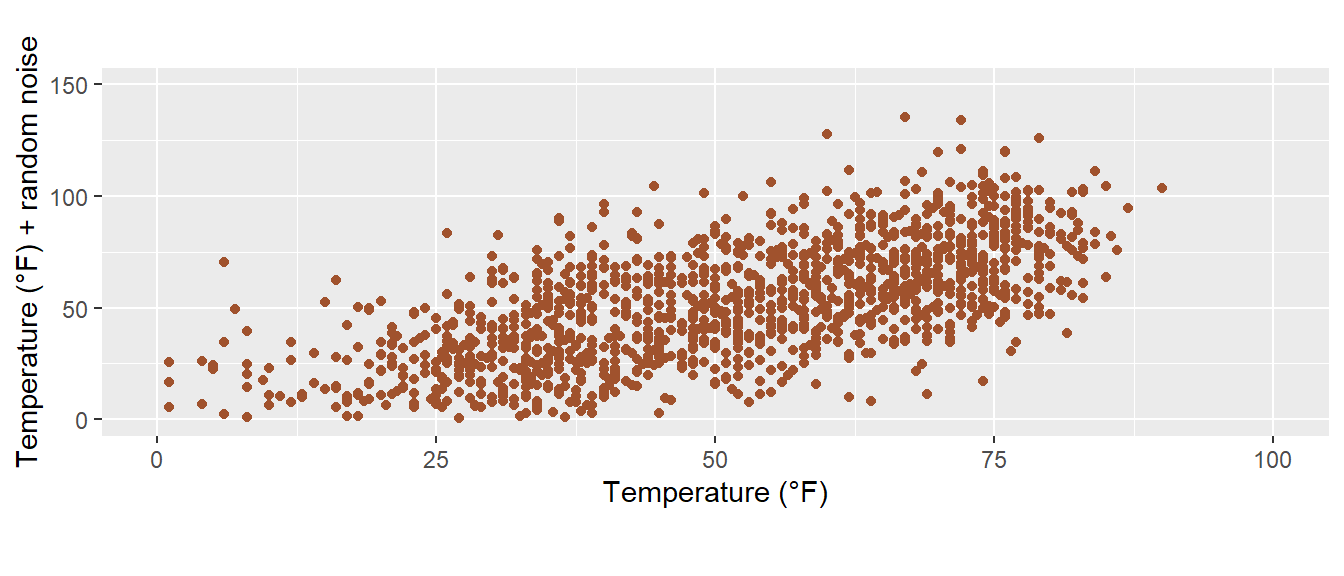
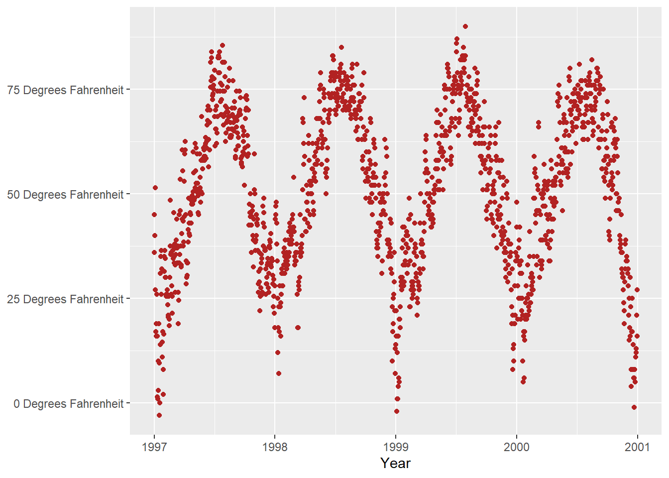
Occasionally, it’s useful to slightly modify your labels, such as adding units or percent signs, without altering your underlying data. You can achieve this using a function:
ggplot(chic, aes(x = date, y = temp)) +
  geom_point(color = "firebrick") +
  labs(x = "Year", y = NULL) +
  scale_y_continuous(label = function(x) {return(paste(x, "Degrees Fahrenheit"))})