ggplot(chic, aes(x = date, y = temp)) +
  geom_point(color = "orangered", alpha = .3) +
  theme(axis.text.x = element_text(angle = 45, vjust = 1, hjust = 1)) +
  labs(x = "Year", y = "Temperature (°F)") +
  facet_grid(year ~ season)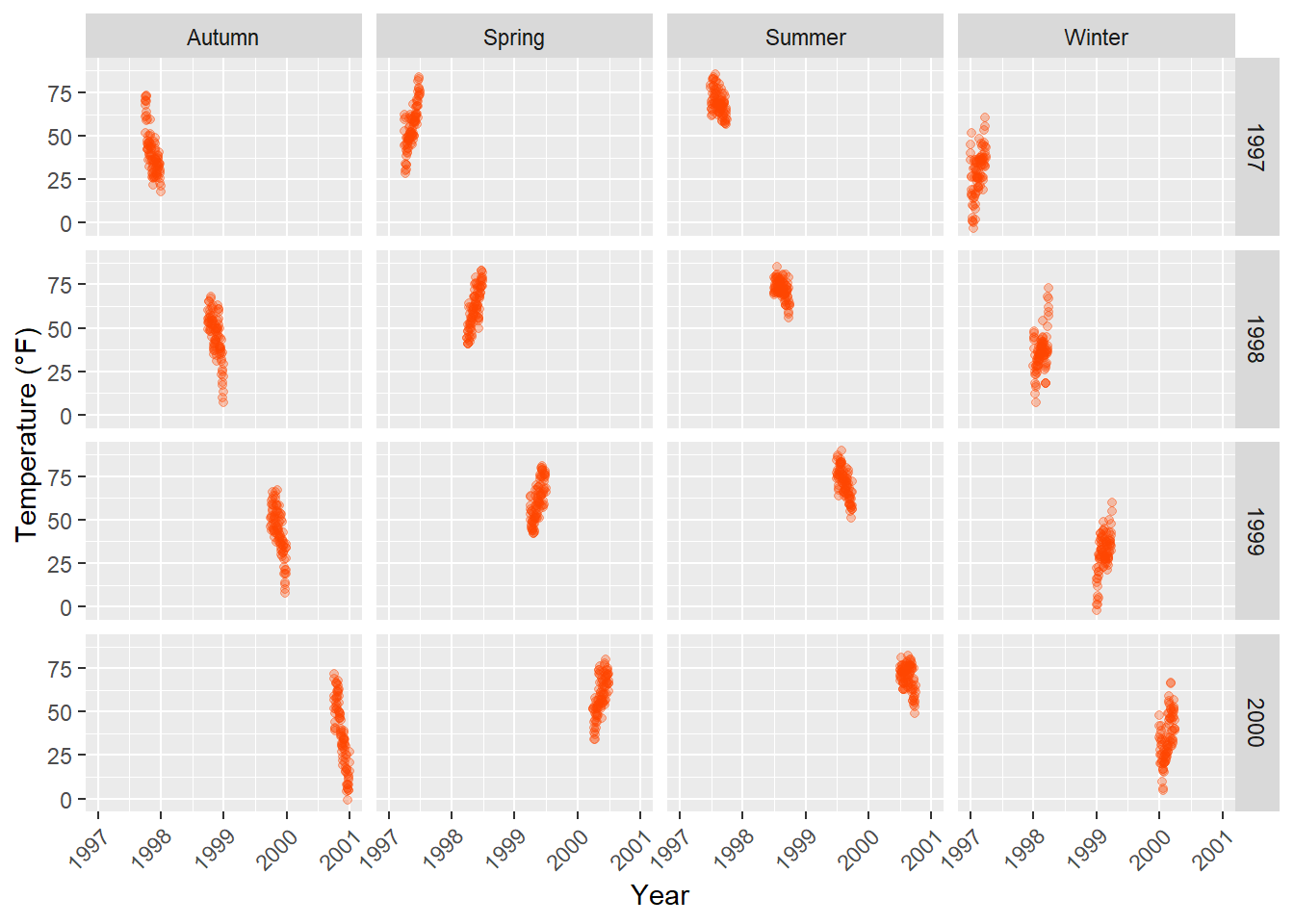
The {ggplot2} package offers two handy functions for creating multi-panel plots, called facets. They are related but have slight differences: facet_wrap creates a ribbon of plots based on a single variable, while facet_grid spans a grid of plots based on two variables.
When dealing with two variables, facet_grid is the appropriate choice. In this function, the order of the variables determines the number of rows and columns in the grid:
ggplot(chic, aes(x = date, y = temp)) +
geom_point(color = "orangered", alpha = .3) +
theme(axis.text.x = element_text(angle = 45, vjust = 1, hjust = 1)) +
labs(x = "Year", y = "Temperature (°F)") +
facet_grid(year ~ season)
To switch from a row-based arrangement to a column-based one, you can modify facet_grid(year ~ season) to facet_grid(season ~ year).
facet_wrap creates a facet of a single variable, specified with a tilde in front: facet_wrap(~ variable). The appearance of these subplots is determined by the arguments ncol and nrow:
g <-
  ggplot(chic, aes(x = date, y = temp)) +
    geom_point(color = "chartreuse4", alpha = .3) +
    labs(x = "Year", y = "Temperature (°F)") +
    theme(axis.text.x = element_text(angle = 45, vjust = 1, hjust = 1))

g + facet_wrap(~ year)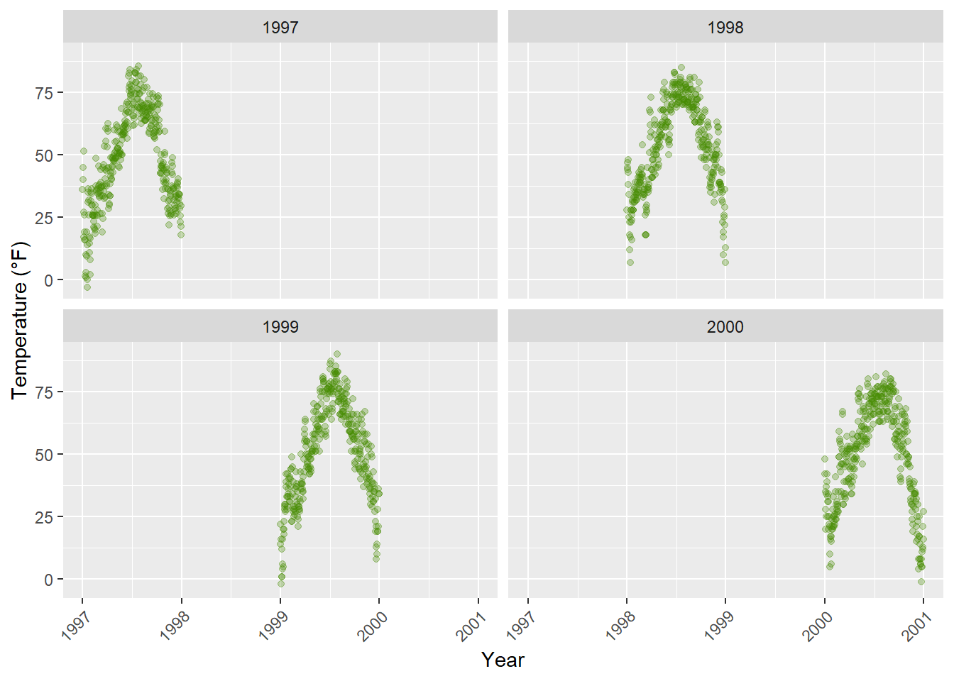
Accordingly, you can arrange the plots as you like, instead as a matrix in one row…
g + facet_wrap(~ year, nrow = 1)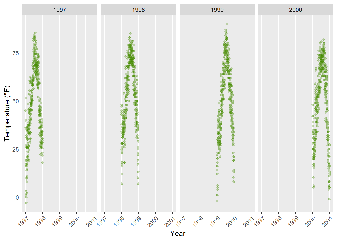
… or even as a asymmetric grid of plots:
g + facet_wrap(~ year, ncol = 3) + theme(axis.title.x = element_text(hjust = .15))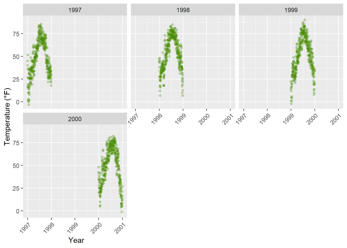
The default for multi-panel plots in {ggplot2} is to use equivalent scales in each panel. But sometimes you want to allow a panels own data to determine the scale. This is often not a good idea since it may give your user the wrong impression about the data. But sometimes it is indeed useful and to do this you can set scales = "free":
g + facet_wrap(~ year, nrow = 2, scales = "free")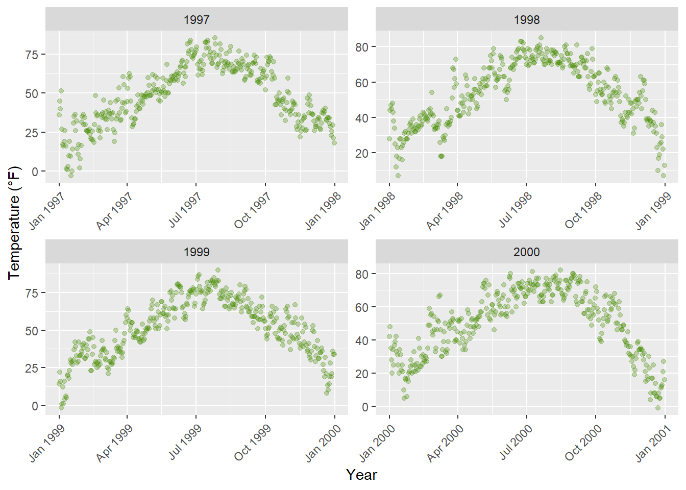
Note that both, x and y axes differ in their range!
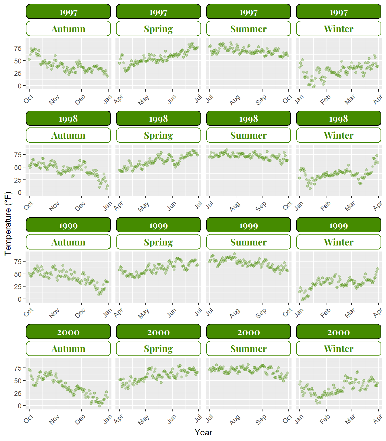
facet_wrap with Two VariablesThe function facet_wrap can also take two variables:
g + facet_wrap(year ~ season, nrow = 4, scales = "free_x")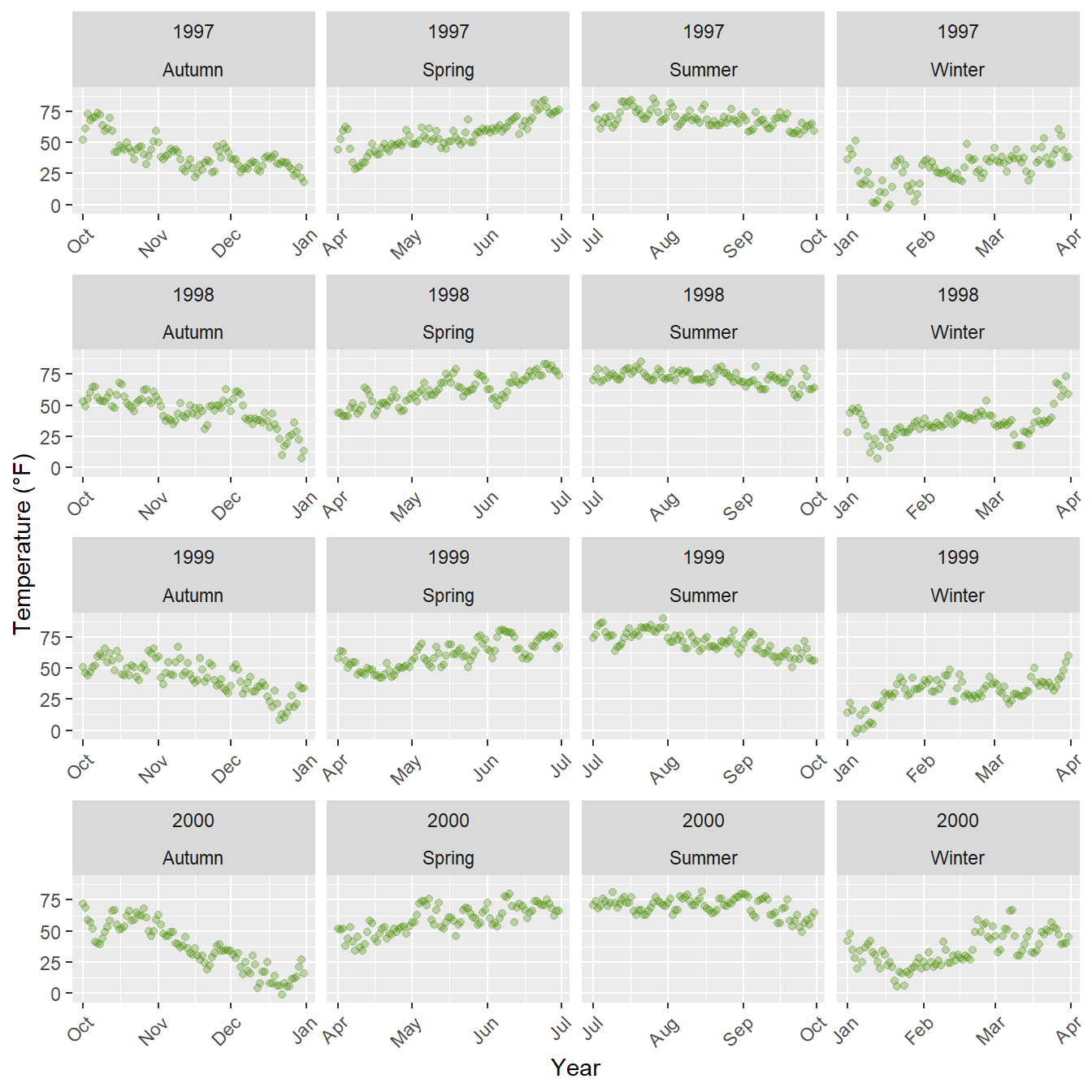
When using facet_wrap you are still able to control the grid design: you can rearrange the number of plots per row and column and you can also let all axes roam free. In contrast, facet_grid will also take a free argument but will only let it roam free per column or row:
g + facet_grid(year ~ season, scales = "free_x")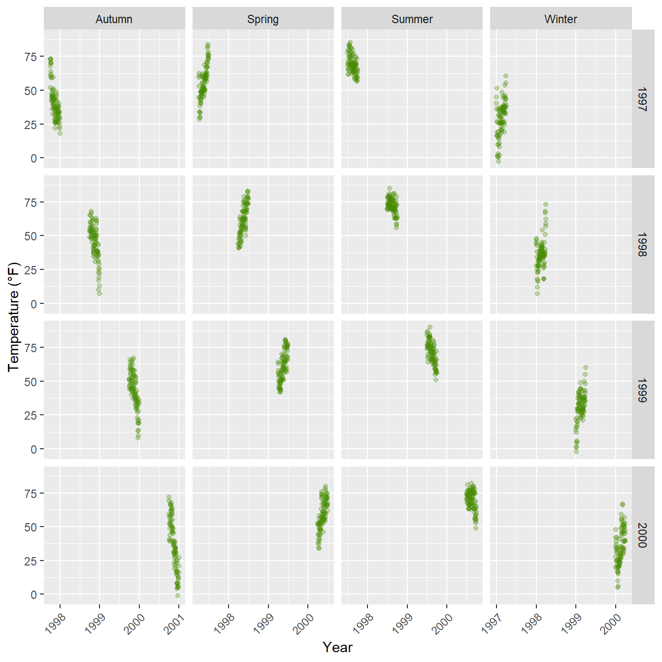
By using theme, you can modify the appearance of the strip text (i.e. the title for each facet) and the strip text boxes:
g + facet_wrap(~ year, nrow = 1, scales = "free_x") +
  theme(strip.text = element_text(face = "bold", color = "chartreuse4",
                                  hjust = 0, size = 20),
        strip.background = element_rect(fill = "chartreuse3", linetype = "dotted"))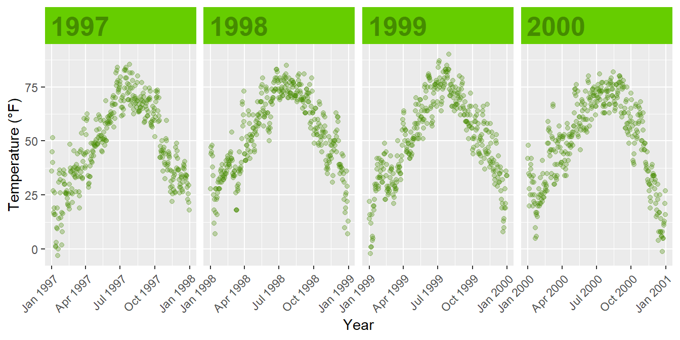
The following two functions adapted from this answer by Claus Wilke, the author of the {ggtext} package, allow to highlight specific labels in combination with element_textbox() that is provided by {ggtext}.
library(ggtext)
library(purrr) ## for %||%

element_textbox_highlight <- function(..., hi.labels = NULL, hi.fill = NULL,
                                      hi.col = NULL, hi.box.col = NULL, hi.family = NULL) {
  structure(
    c(element_textbox(...),
      list(hi.labels = hi.labels, hi.fill = hi.fill, hi.col = hi.col, hi.box.col = hi.box.col, hi.family = hi.family)
    ),
    class = c("element_textbox_highlight", "element_textbox", "element_text", "element")
  )
}

element_grob.element_textbox_highlight <- function(element, label = "", ...) {
  if (label %in% element$hi.labels) {
    element$fill <- element$hi.fill %||% element$fill
    element$colour <- element$hi.col %||% element$colour
    element$box.colour <- element$hi.box.col %||% element$box.colour
    element$family <- element$hi.family %||% element$family
  }
  NextMethod()
}
Now you can use it and specify for example all striptexts:
g + facet_wrap(year ~ season, nrow = 4, scales = "free_x") +
  theme(
    strip.background = element_blank(),
    strip.text = element_textbox_highlight(
      family = "Playfair Display", size = 12, face = "bold",
      fill = "white", box.color = "chartreuse4", color = "chartreuse4",
      halign = .5, linetype = 1, r = unit(5, "pt"), width = unit(1, "npc"),
      padding = margin(5, 0, 3, 0), margin = margin(0, 1, 3, 1),
      hi.labels = c("1997", "1998", "1999", "2000"),
      hi.fill = "chartreuse4", hi.box.col = "black", hi.col = "white"
    )
  )
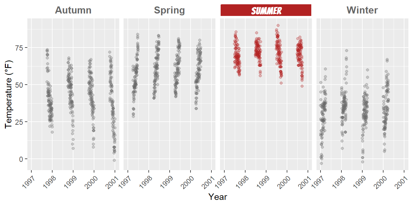
ggplot(chic, aes(x = date, y = temp)) +
  geom_point(aes(color = season == "Summer"), alpha = .3) +
  labs(x = "Year", y = "Temperature (°F)") +
  facet_wrap(~ season, nrow = 1) +
  scale_color_manual(values = c("gray40", "firebrick"), guide = "none") +
  theme(
    axis.text.x = element_text(angle = 45, vjust = 1, hjust = 1),
    strip.background = element_blank(),
    strip.text = element_textbox_highlight(
      size = 12, face = "bold",
      fill = "white", box.color = "white", color = "gray40",
      halign = .5, linetype = 1, r = unit(0, "pt"), width = unit(1, "npc"),
      padding = margin(2, 0, 1, 0), margin = margin(0, 1, 3, 1),
      hi.labels = "Summer", hi.family = "Bangers",
      hi.fill = "firebrick", hi.box.col = "firebrick", hi.col = "white"
    )
  )
There are several ways how plots can be combined. The easiest approach in my opinion is the {patchwork} package by Thomas Lin Pedersen:
p1 <- ggplot(chic, aes(x = date, y = temp,
                       color = season)) +
        geom_point() +
        geom_rug() +
        labs(x = "Year", y = "Temperature (°F)")

p2 <- ggplot(chic, aes(x = date, y = o3)) +
        geom_line(color = "gray") +
        geom_point(color = "darkorange2") +
        labs(x = "Year", y = "Ozone")

library(patchwork)
p1 + p2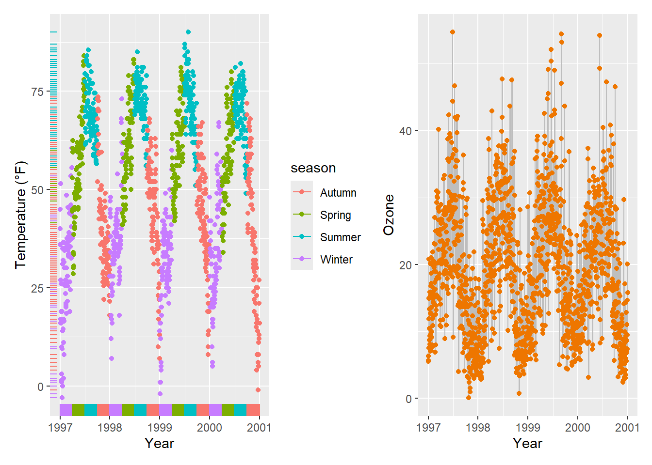
We can change the order by “dividing” both plots (and note the alignment even though one has a legend and one doesn’t!):
p1 / p2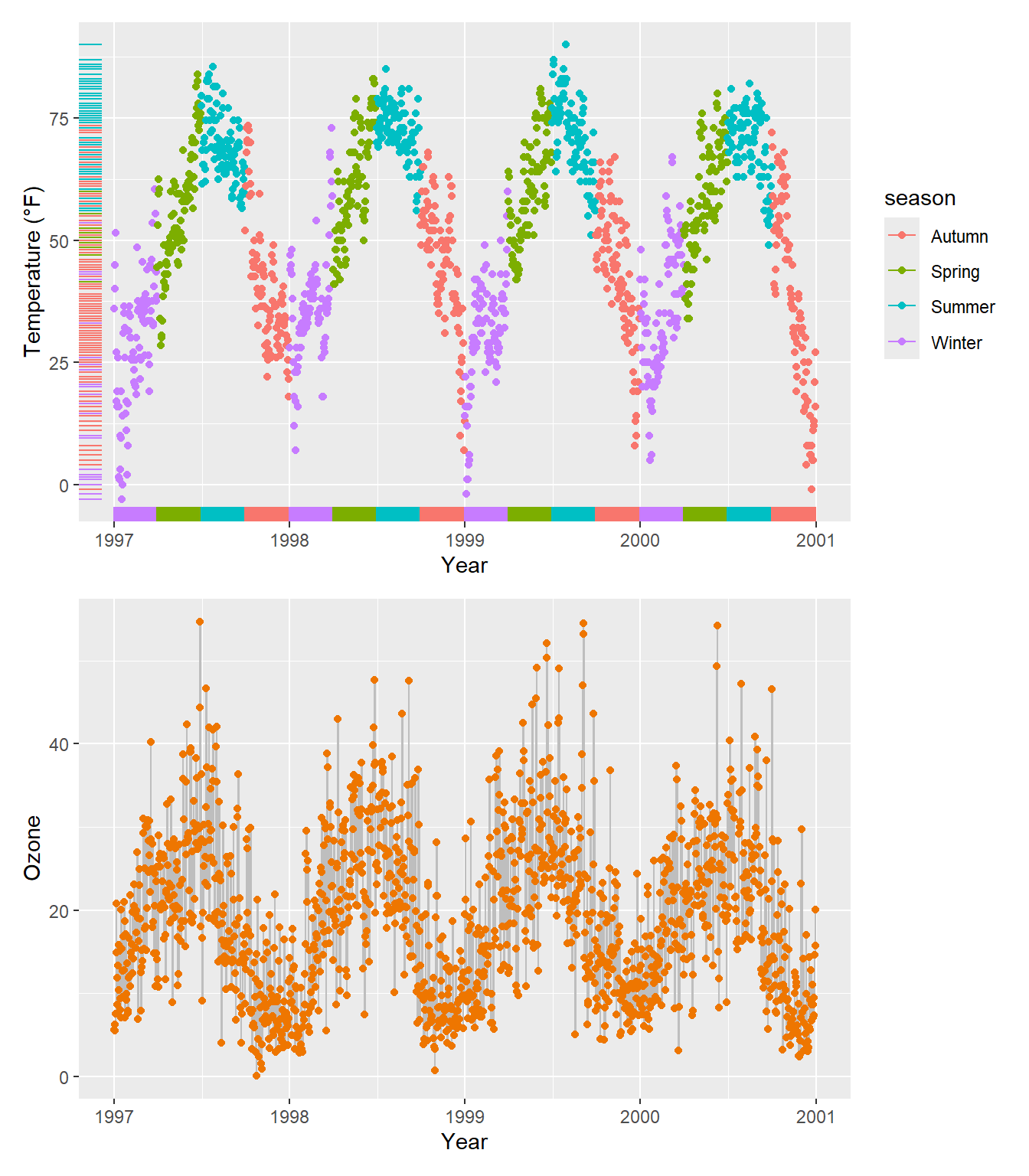
And also nested plots are possible!
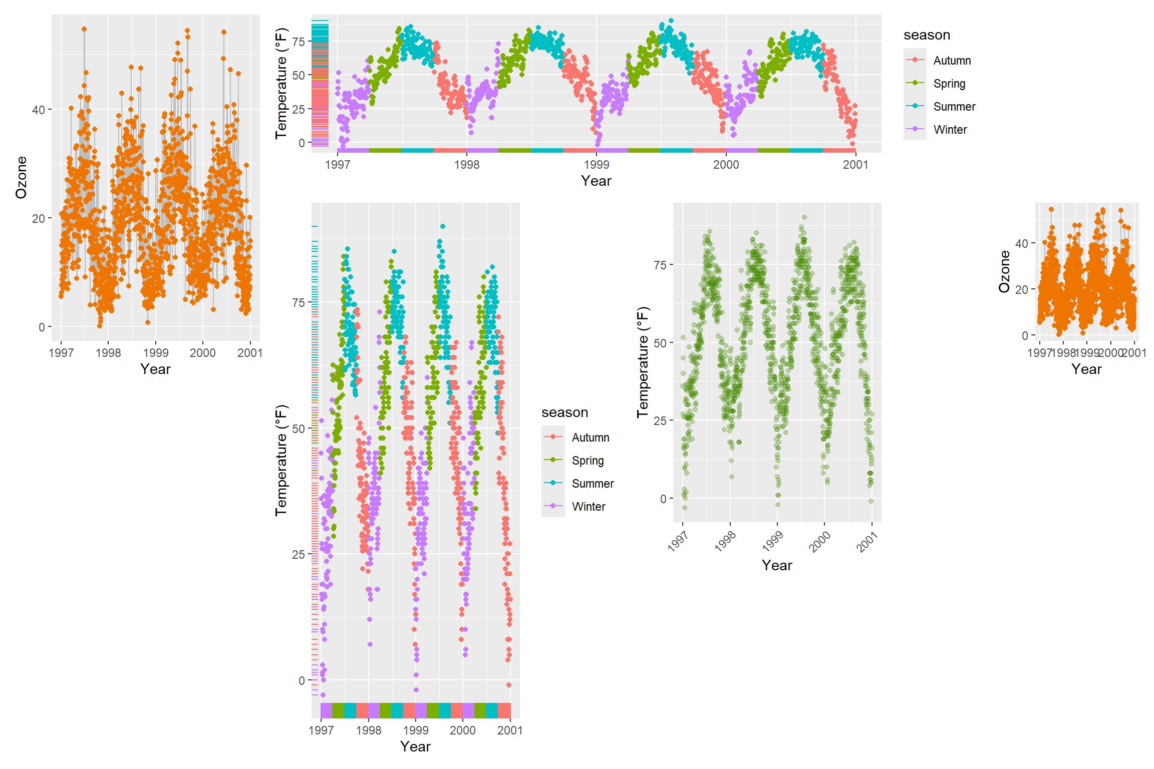
(g + p2) / p1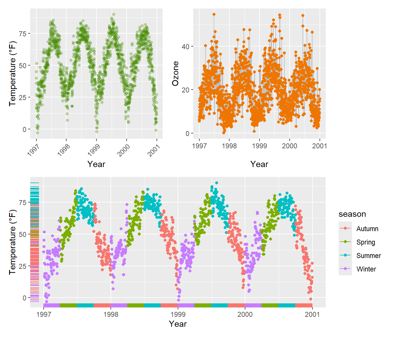
(Note the alignment of the plots even though only one plot includes a legend.)
Alternatively, the {cowplot} package by Claus Wilke provides the functionality to combine multiple plots (and lots of other good utilities):
library(cowplot)
Attaching package: 'cowplot'The following object is masked from 'package:patchwork':
align_plotsThe following object is masked from 'package:lubridate':
stampplot_grid(plot_grid(g, p1), p2, ncol = 1)
… and so does the {gridExtra} package as well:
library(gridExtra)
Attaching package: 'gridExtra'The following object is masked from 'package:dplyr':
combinegrid.arrange(g, p1, p2,
layout_matrix = rbind(c(1, 2), c(3, 3)))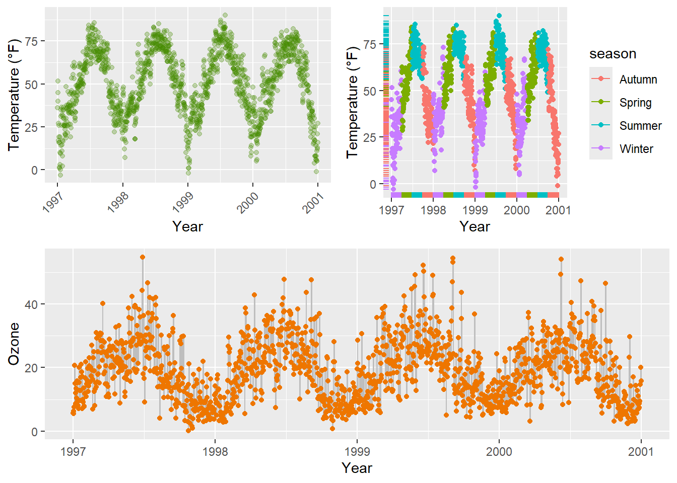
The same idea of defining a layout can be used with {patchwork} which allows creating complex compositions:
layout <- "
AABBBB#
AACCDDE
##CCDD#
##CC###
"

p2 + p1 + p1 + g + p2 +
  plot_layout(design = layout)