rayshader is an open source package for producing 2D and 3D data visualizations in R. rayshader uses elevation data in a base R matrix and a combination of raytracing, hillshading algorithms, and overlays to generate stunning 2D and 3D maps. In addition to maps, rayshader also allows the user to translate ggplot2 objects into beautiful 3D data visualizations.
The models can be rotated and examined interactively or the camera movement can be scripted to create animations. Scenes can also be rendered using a high-quality pathtracer, rayrender. The user can also create a cinematic depth of field post-processing effect to direct the user’s focus to important regions in the figure. The 3D models can also be exported to a 3D-printable format with a built-in STL export function, and can be exported to an OBJ file for use in other 3D modeling software. rayshader is a powerful tool for creating 3D visualizations of data, and can be used to create stunning visualizations for scientific research, data analysis, and art. You can find more information about rayshader at https://www.rayshader.com/.
Let’s see some 3D plots using rayshader.
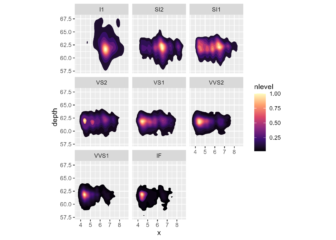
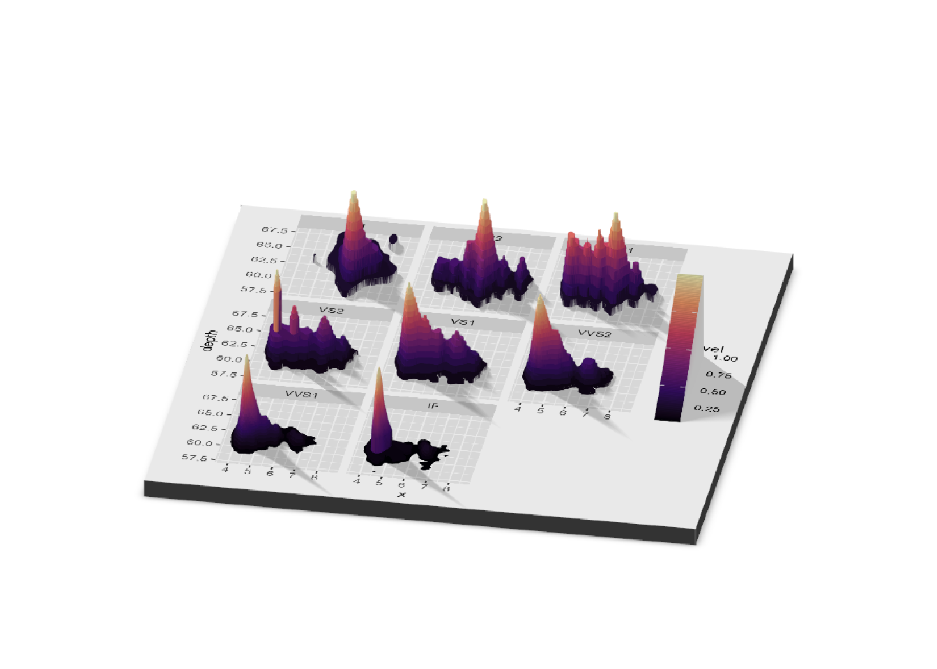
library(ggplot2)library(rayshader)ggdiamonds =ggplot(diamonds) +stat_density_2d(aes(x = x, y = depth, fill =after_stat(nlevel)), geom ="polygon", n =200, bins =50,contour =TRUE) +facet_wrap(clarity~.) +scale_fill_viridis_c(option ="A")plot_gg(ggdiamonds, width =5, height =5, raytrace =FALSE, preview =TRUE)
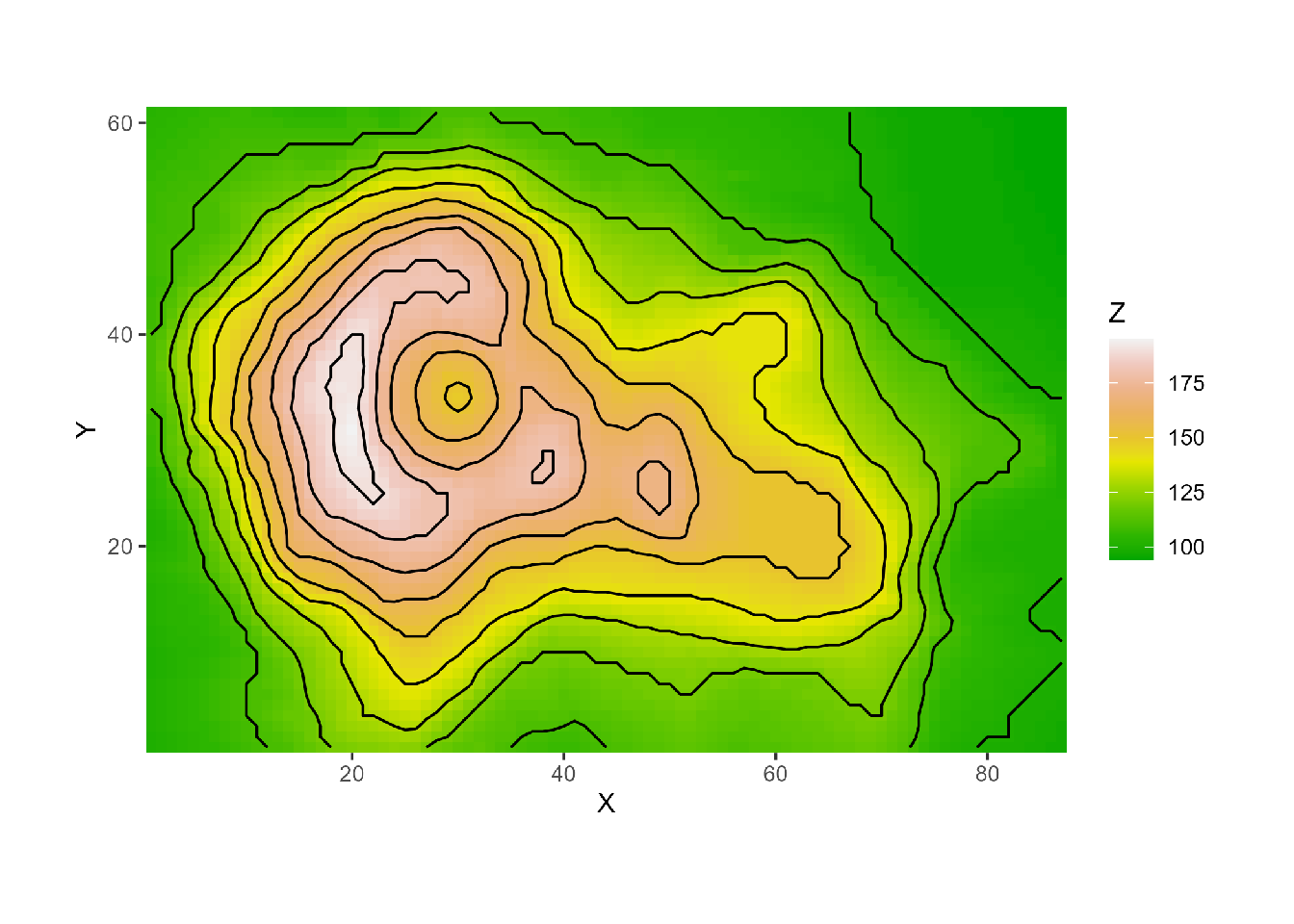
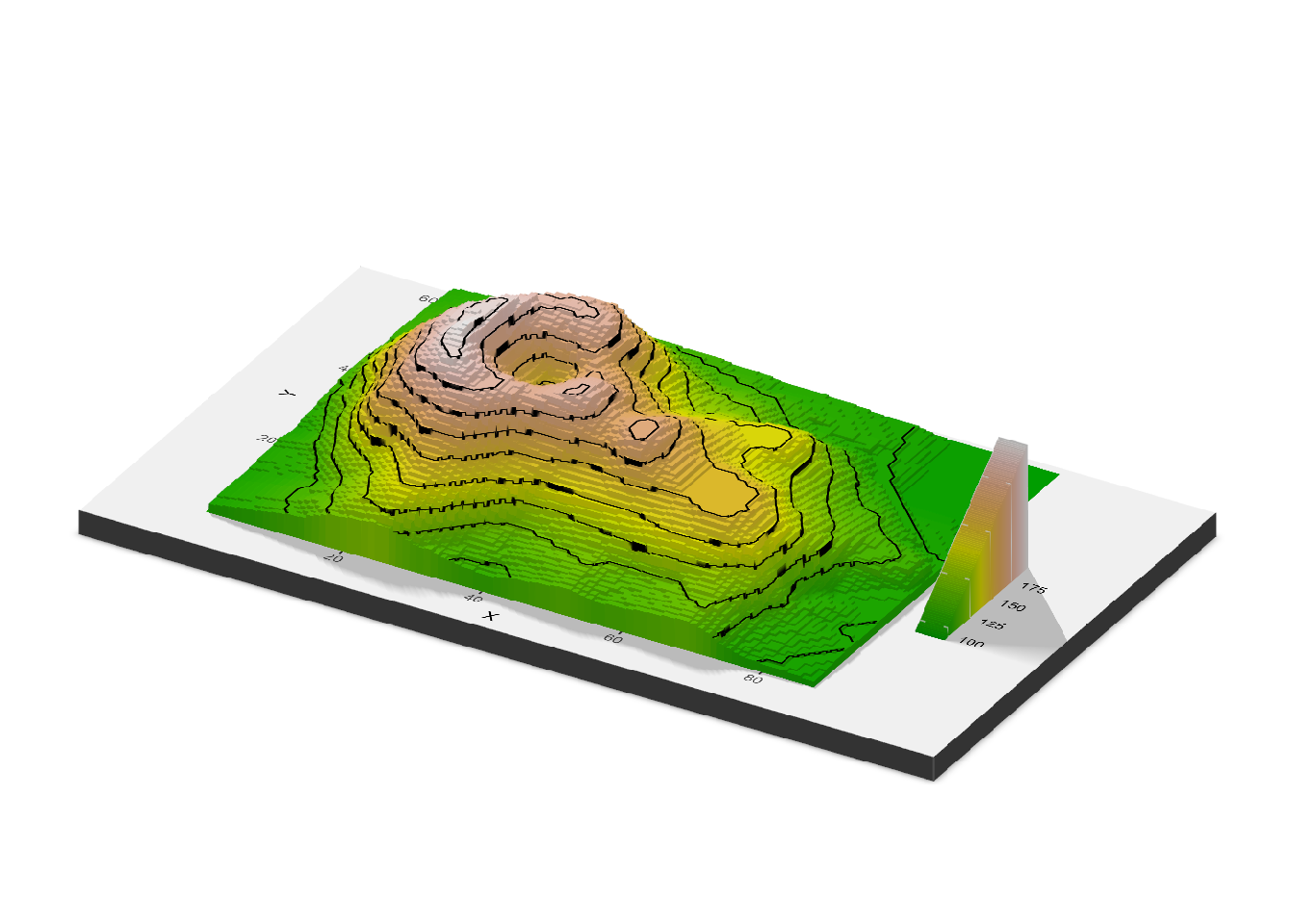
Rayshader will automatically ignore lines and other elements that should not be mapped to 3D. Here’s a contour plot of the volcano dataset.
library(reshape2)#Contours and other lines will automatically be ignored. Here is the volcano dataset:ggvolcano = volcano %>%melt() %>%ggplot() +geom_tile(aes(x = Var1, y = Var2, fill = value)) +geom_contour(aes(x = Var1, y = Var2, z = value), color ="black") +scale_x_continuous("X", expand =c(0, 0)) +scale_y_continuous("Y", expand =c(0, 0)) +scale_fill_gradientn("Z", colours =terrain.colors(10)) +coord_fixed()par(mfrow =c(1, 2))plot_gg(ggvolcano, width =7, height =4, raytrace =FALSE, preview =TRUE)
Warning: Removed 1861 rows containing missing values or values outside the scale range
(`geom_contour()`).
Warning: Removed 1861 rows containing missing values or values outside the scale range
(`geom_contour()`).
Sys.sleep(0.2)render_snapshot(clear =TRUE)
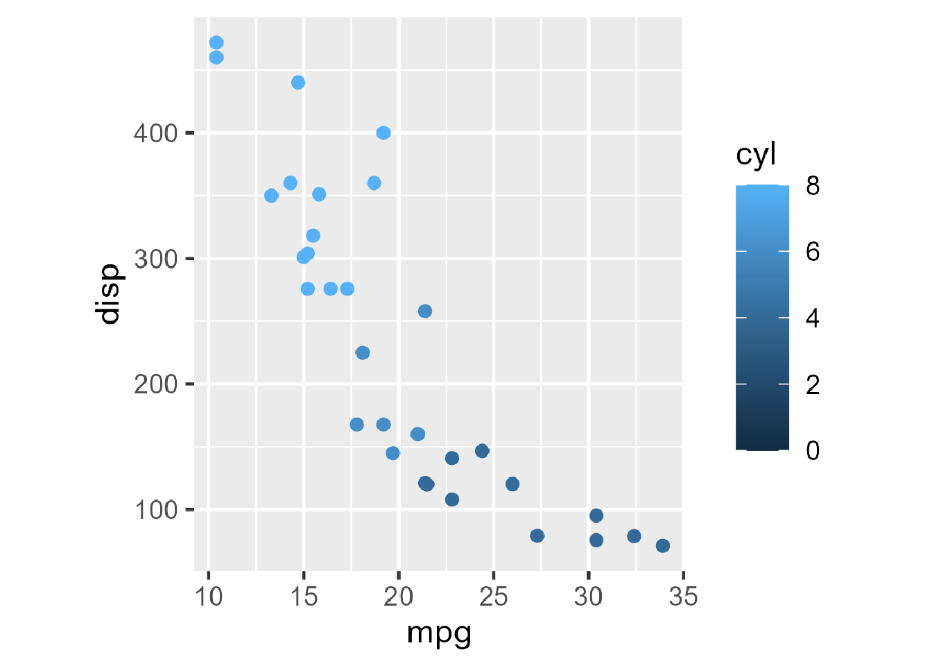
Rayshader also detects when the user passes the color aesthetic, and maps those values to 3D. If both color and fill are passed, however, rayshader will default to fill.
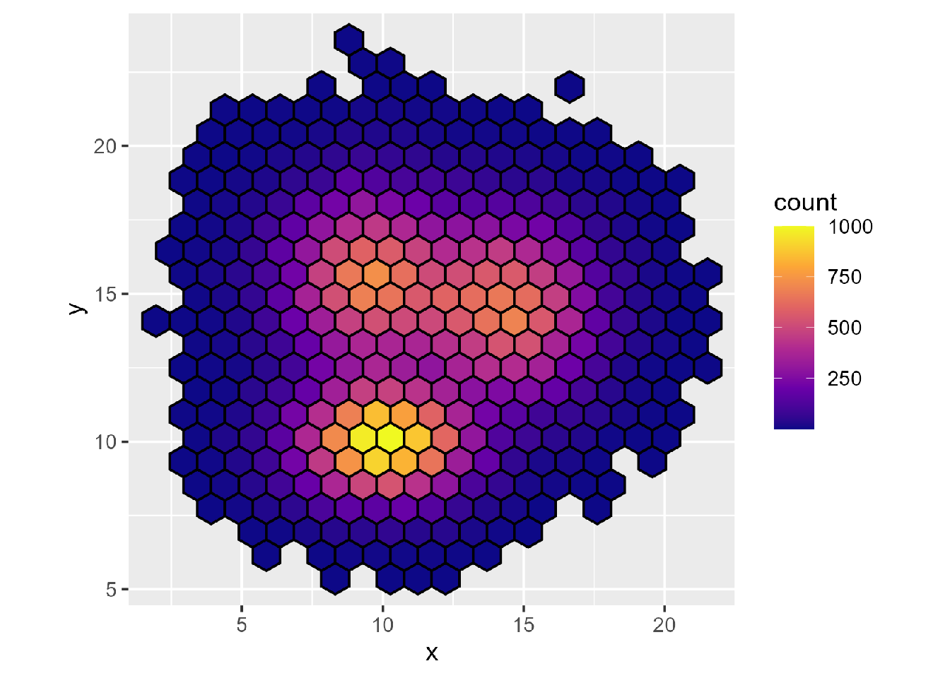
Utilize combinations of line color and fill to create different effects. Here is a terraced hexbin plot, created by mapping the line colors of the hexagons to black.
a =data.frame(x =rnorm(20000, 10, 1.9), y =rnorm(20000, 10, 1.2))b =data.frame(x =rnorm(20000, 14.5, 1.9), y =rnorm(20000, 14.5, 1.9))c =data.frame(x =rnorm(20000, 9.5, 1.9), y =rnorm(20000, 15.5, 1.9))data =rbind(a, b, c)#Lineslibrary(hexbin)pp =ggplot(data, aes(x = x, y = y)) +geom_hex(bins =20, size =0.5, color ="black") +scale_fill_viridis_c(option ="C")
Warning: Using `size` aesthetic for lines was deprecated in ggplot2 3.4.0.
ℹ Please use `linewidth` instead.
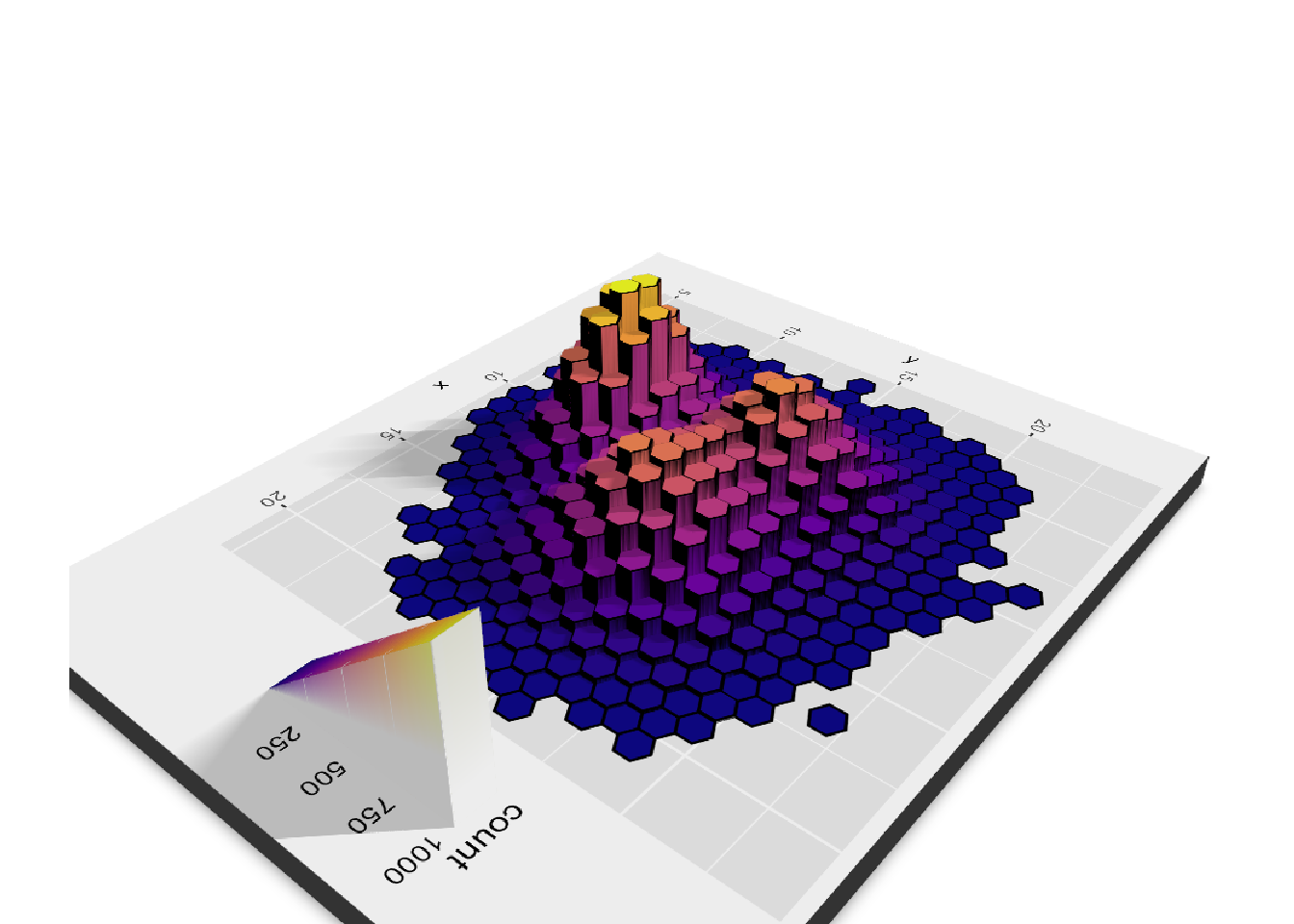
Pretty cool, right? You can create stunning 3D visualizations using rayshader. You can find more information about rayshader at https://www.rayshader.com/.
We can also Use rayshader to create 3D maps. That will be whole another book, we’ll publish that soon. Stay tuned!