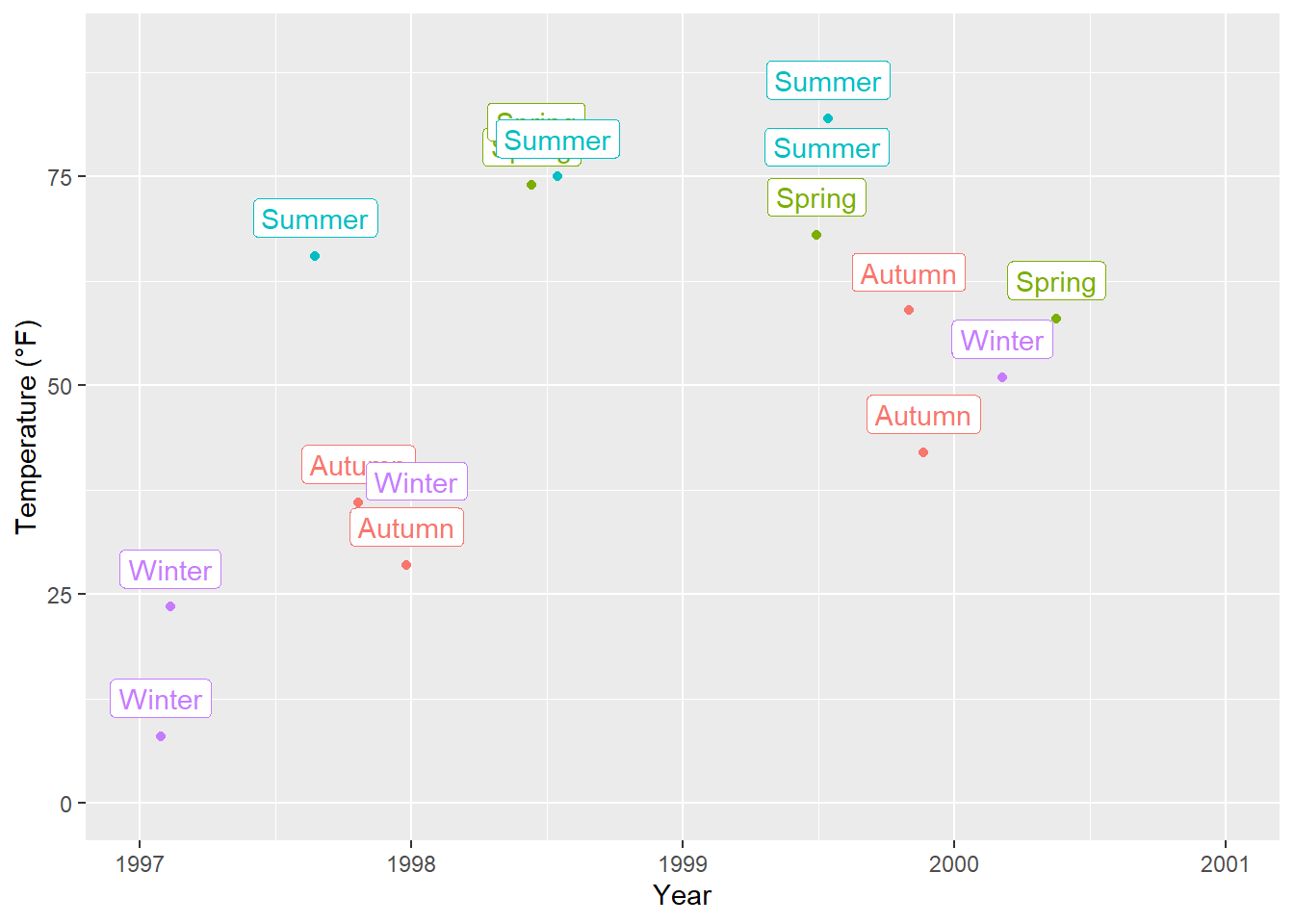
Sometimes, we want to label our data points. To avoid overlaying and crowding by text labels, we use a 1% sample of the original data, equally representing the four seasons. We are using geom_label() which comes with a new aesthetic called label:
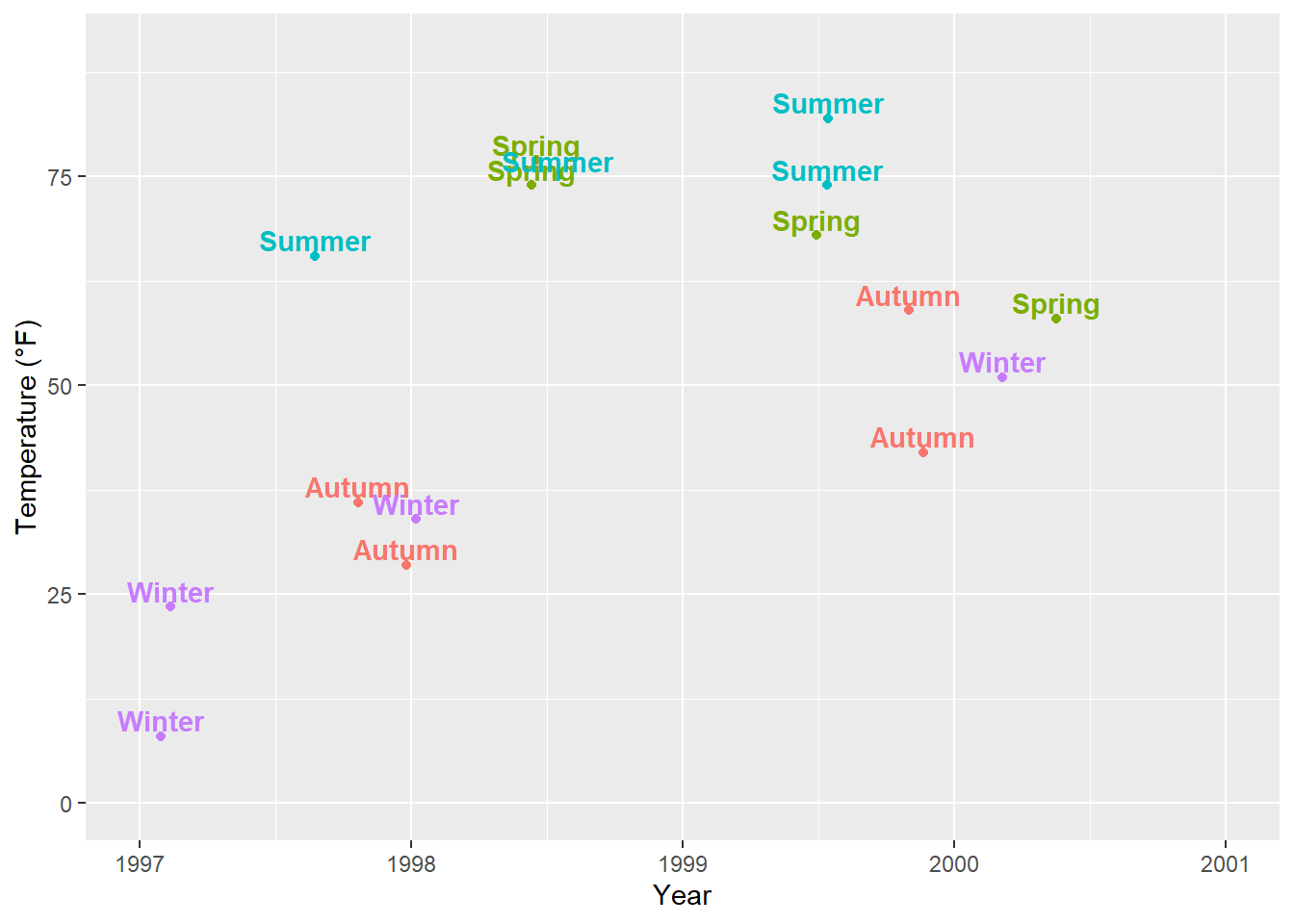
The {ggrepel} package offers some great utilities by providing geoms for {ggplot2} to repel overlapping text as in our examples above. We simply replace geom_text() by geom_text_repel() and geom_label() by geom_label_repel():
library(ggrepel)ggplot(sample, aes(x = date, y = temp, color = season)) +geom_point() +geom_label_repel(aes(label = season), fontface ="bold") +labs(x ="Year", y ="Temperature (°F)") +theme(legend.position ="none")
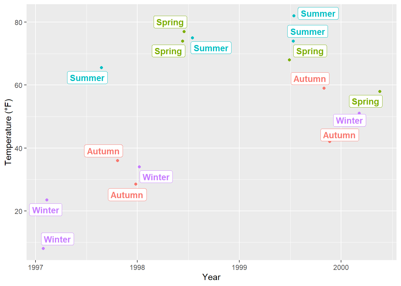
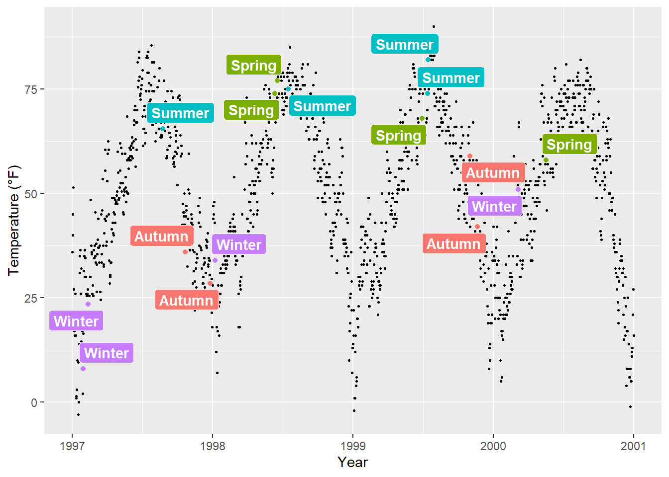
It may look nicer with filled boxes so we map season to fill instead to color and set a white color for the text:
This also works for the pure text labels by using geom_text_repel(). Have a look at all the usage examples.
13.2 Add Text Annotations
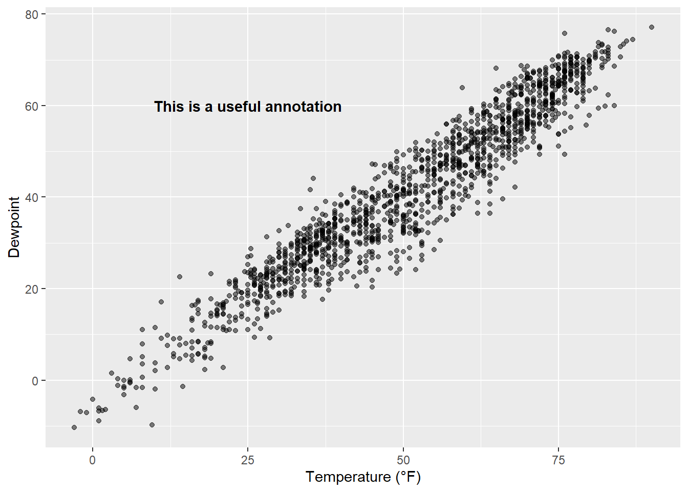
There are several ways how one can add annotations to a ggplot. We can again use annotate(geom = "text"), annotate(geom = "label"), geom_text() or geom_label():
g <-ggplot(chic, aes(x = temp, y = dewpoint)) +geom_point(alpha = .5) +labs(x ="Temperature (°F)", y ="Dewpoint")g +annotate(geom ="text", x =25, y =60, fontface ="bold", label ="This is a useful annotation")
However, now ggplot has drawn one text label per data point—that’s 1,461 labels and you only see one! You can solve that by setting the stat argument to "unique":
g +geom_text(aes(x =25, y =60,label ="This is a useful annotation"),stat ="unique")
Warning in geom_text(aes(x = 25, y = 60, label = "This is a useful annotation"), : All aesthetics have length 1, but the data has 1461 rows.
ℹ Please consider using `annotate()` or provide this layer with data containing
  a single row.
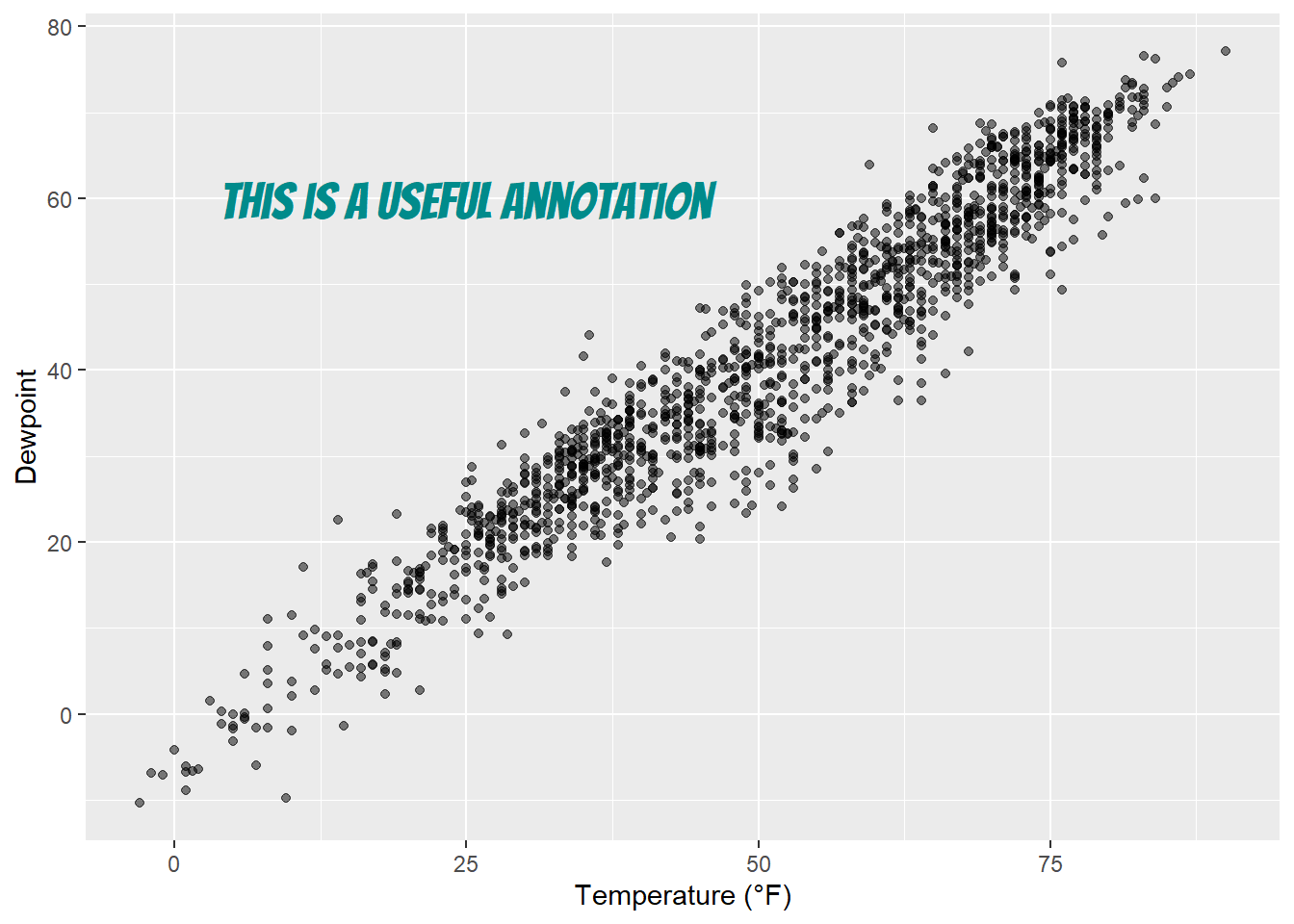
By the way, of course one can change the properties of the displayed text:
g +geom_text(aes(x =25, y =60,label ="This is a useful annotation"),stat ="unique", family ="Bangers",size =7, color ="darkcyan")
Warning in geom_text(aes(x = 25, y = 60, label = "This is a useful annotation"), : All aesthetics have length 1, but the data has 1461 rows.
ℹ Please consider using `annotate()` or provide this layer with data containing
  a single row.
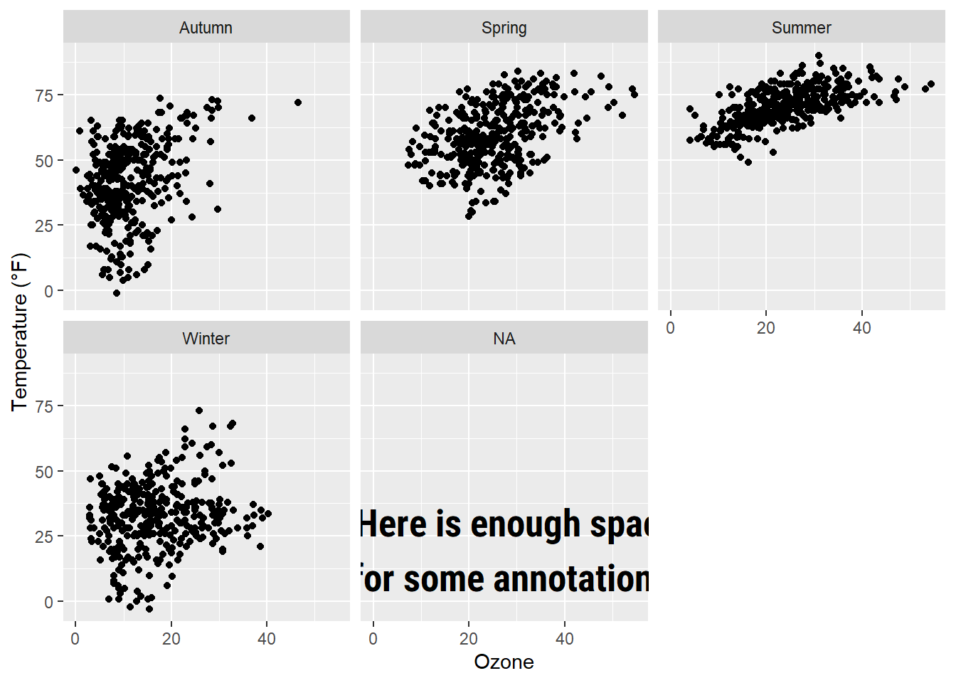
In case you use one of the facet functions to visualize your data you might run into trouble. One thing is that you may want to include the annotation only once:
ann <-data.frame(o3 =30,temp =20,season =factor("Summer", levels =levels(chic$season)),label ="Here is enough space\nfor some annotations.")g <-ggplot(chic, aes(x = o3, y = temp)) +geom_point() +labs(x ="Ozone", y ="Temperature (°F)")g +geom_text(data = ann, aes(label = label),size =7, fontface ="bold",family ="Roboto Condensed") +facet_wrap(~season)
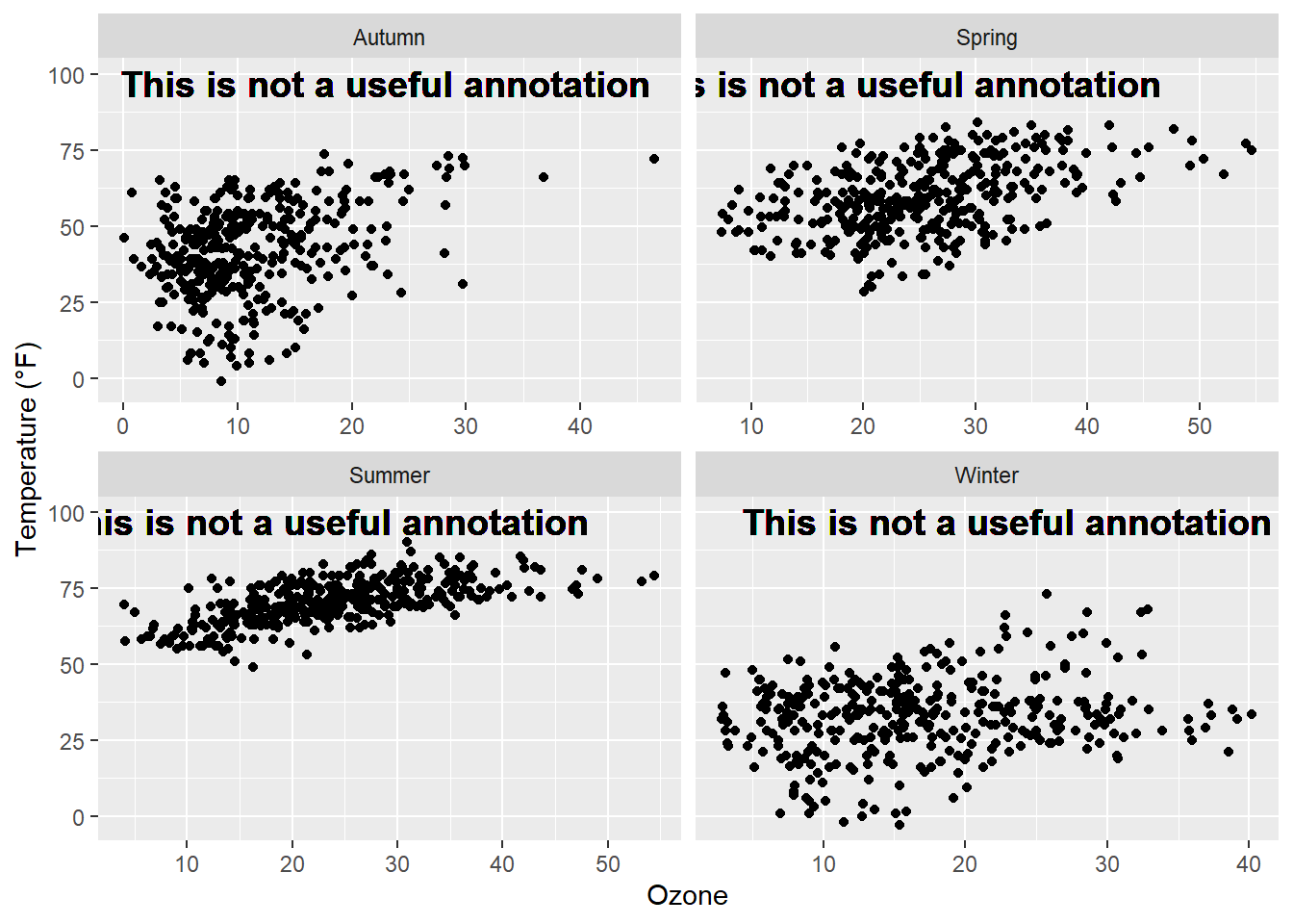
Another challenge are facets in combination with free scales that might cut your text:
g +geom_text(aes(x =23, y =97,label ="This is not a useful annotation"),size =5, fontface ="bold") +scale_y_continuous(limits =c(NA, 100)) +facet_wrap(~season, scales ="free_x")
Warning in geom_text(aes(x = 23, y = 97, label = "This is not a useful annotation"), : All aesthetics have length 1, but the data has 1461 rows.
ℹ Please consider using `annotate()` or provide this layer with data containing
  a single row.
One solution is to calculate the midpoint of the axis, here x, beforehand:
# A tibble: 4 × 2
  season    o3
  <chr>  <dbl>
1 Autumn  23.3
2 Spring  31.0
3 Summer  29.2
4 Winter  21.5
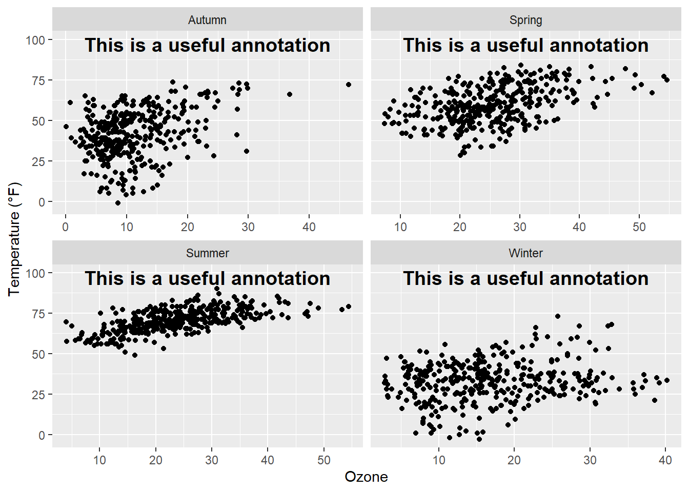
… and use the aggreated data to specify the placement of the annotation:
g +geom_text(data = ann,aes(x = o3, y =97,label ="This is a useful annotation"),size =5, fontface ="bold") +scale_y_continuous(limits =c(NA, 100)) +facet_wrap(~season, scales ="free_x")
However, there is a simpler approach (in terms of fixing the cordinates)—but it also takes a while to know the code by heart. The {grid} package in combination with {ggplot2}’s annotation_custom() allows you to specify the location based on scaled coordinates where 0 is low and 1 is high. grobTree() creates a grid graphical object and textGrob creates the text graphical object. The value of this is particularly evident when you have multiple plots with different scales.
library(grid)my_grob <-grobTree(textGrob("This text stays in place!",x = .1, y = .9, hjust =0,gp =gpar(col ="black",fontsize =15,fontface ="bold")))g +annotation_custom(my_grob) +facet_wrap(~season, scales ="free_x") +scale_y_continuous(limits =c(NA, 100))
13.3 Use Markdown and HTML Rendering for Annotations
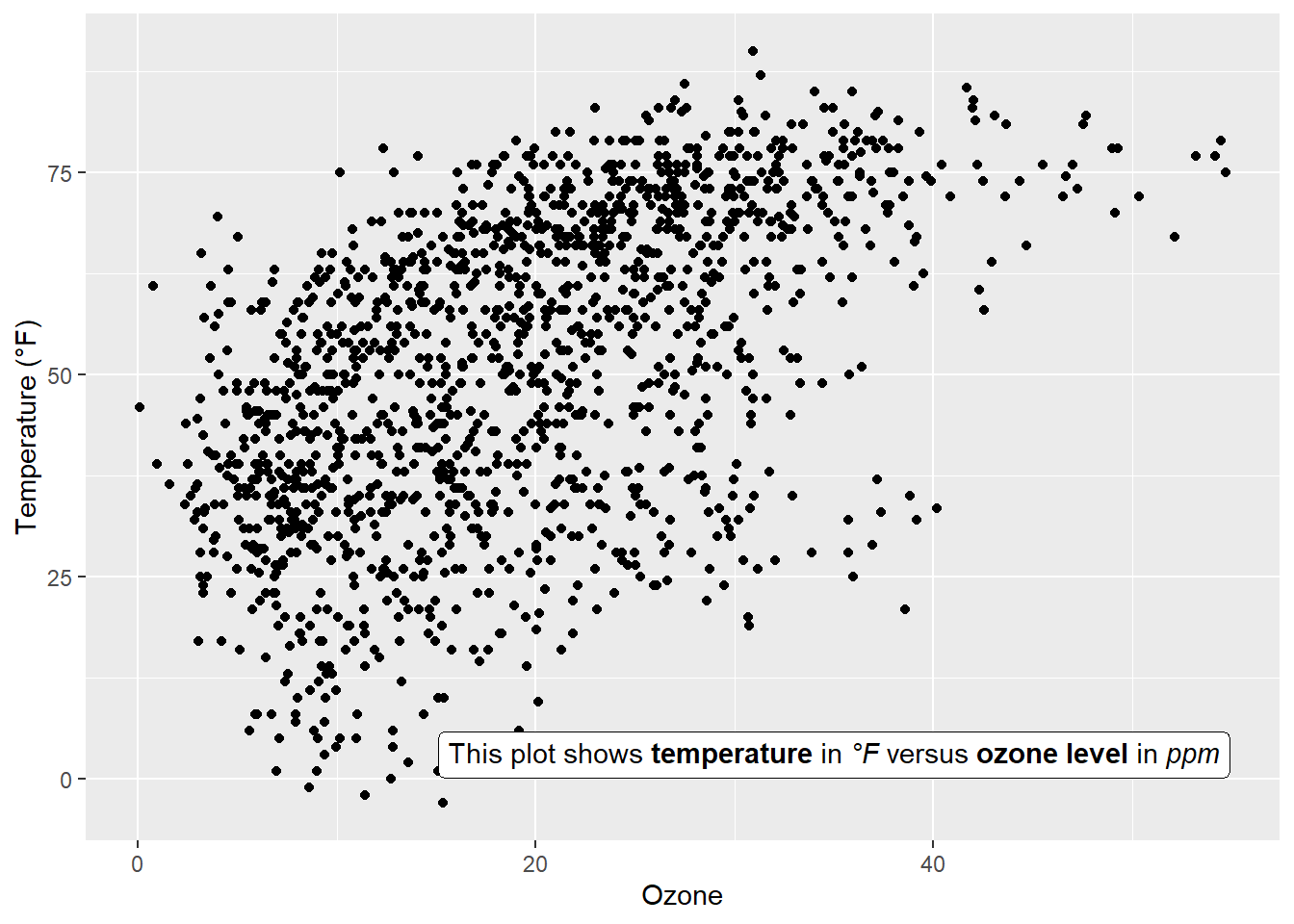
Again, we are using Claus Wilke’s {ggtext} package that is designed for improved text rendering support for {ggplot2}. The {ggtext} package defines two new theme elements, element_markdown() and element_textbox(). The package also provides additional geoms. geom_richtext() is a replacement for geom_text() and geom_label() and renders text as markdown…
library(ggtext)lab_md <-"This plot shows **temperature** in *°F* versus **ozone level** in *ppm*"g +geom_richtext(aes(x =35, y =3, label = lab_md),stat ="unique")
Warning in geom_richtext(aes(x = 35, y = 3, label = lab_md), stat = "unique"): All aesthetics have length 1, but the data has 1461 rows.
ℹ Please consider using `annotate()` or provide this layer with data containing
  a single row.
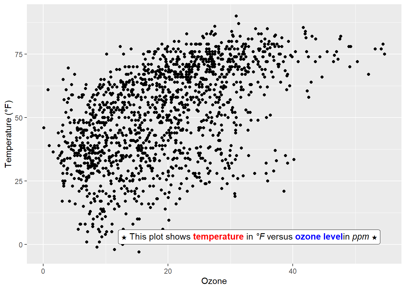
… or html:
lab_html <-"★ This plot shows <b style='color:red;'>temperature</b> in <i>°F</i> versus <b style='color:blue;'>ozone level</b>in <i>ppm</i> ★"g +geom_richtext(aes(x =33, y =3, label = lab_html),stat ="unique")
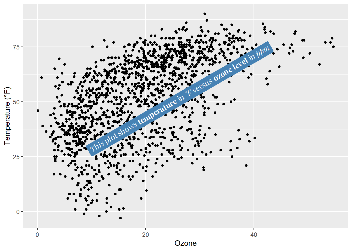
The geom comes with a lot of details one can modify, such as angle (which is not possible in the default geom_text() and geom_label()), properties of the box and properties of the text.
g +geom_richtext(aes(x =10, y =25, label = lab_md),stat ="unique", angle =30,color ="white", fill ="steelblue",label.color =NA, hjust =0, vjust =0,family ="Playfair Display")
Warning in geom_richtext(aes(x = 10, y = 25, label = lab_md), stat = "unique", : All aesthetics have length 1, but the data has 1461 rows.
ℹ Please consider using `annotate()` or provide this layer with data containing
  a single row.
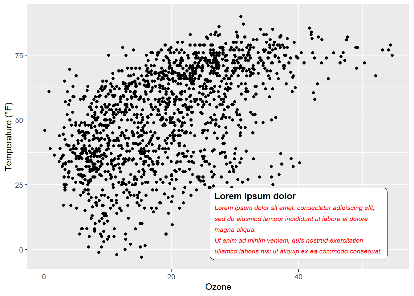
The other geom from the {ggtext} package is geom_textbox(). This geom allows for dynamic wrapping of strings which is very useful for longer annotations such as info boxes and subtitles.
lab_long <-"**Lorem ipsum dolor**<br><i style='font-size:8pt;color:red;'>Lorem ipsum dolor sit amet, consectetur adipiscing elit, sed do eiusmod tempor incididunt ut labore et dolore magna aliqua.<br>Ut enim ad minim veniam, quis nostrud exercitation ullamco laboris nisi ut aliquip ex ea commodo consequat.</i>"g +geom_textbox(aes(x =40, y =10, label = lab_long),width =unit(15, "lines"), stat ="unique")
Warning in geom_textbox(aes(x = 40, y = 10, label = lab_long), width = unit(15, : All aesthetics have length 1, but the data has 1461 rows.
ℹ Please consider using `annotate()` or provide this layer with data containing
  a single row.
Note that it is not possible to either rotate the textbox (always horizontal) nor to change the justification of the text (always left-aligned).